Overview
This document demonstrates how to generate random sampling points within a polygon while enforcing a minimum distance between points using a Simple Sequential Inhibition (SSI) process.
Libraries
library(sf)
library(spatstat.geom)
library(spatstat.random)
library(dplyr)
library(ggplot2)
library(maptiles)
library(ggspatial)
library(units)
We load:
sffor modern spatial data handlingspatstatmodules for generating spatial point patternsggplot2for plottingmaptilesandggspatialfor modern basemaps and map annotationsunitsto safely handle distance units (e.g. metres)
First, create a bounding polygon using longitude and latitude coordinates in the WGS84 coordinate system. While this format is convenient for defining locations, it is not suitable for measuring distances because the units are in degrees rather than metres. To address this, the polygon is reprojected into the British National Grid coordinate system (EPSG:27700), which uses metres as its unit. This transformation is essential for ensuring that the minimum distance constraint applied later is accurate and interpretable. You can of course use our own shapefile if you don’t want to manually create a bounding polygon.
spatstat uses its own internal representation of space called an “observation window” (owin). We convert the sf polygon into owin format so it can be used as the boundary within which points will be generated. Without this conversion, the simulation functions in spatstat would not recognise the study area.
x <- c(-3.541238, -3.547341, -3.561397, -3.572132, -3.572495, -3.551687,
       -3.566528, -3.599789, -3.592162, -3.604156, -3.629145, -3.618190,
       -3.585571, -3.572779, -3.525398, -3.504483, -3.525454, -3.541238)

y <- c(51.68106, 51.69050, 51.7003, 51.69617, 51.68800, 51.67405,
       51.64949, 51.65832, 51.67560, 51.68177, 51.71373, 51.72463,
       51.73346, 51.73788, 51.71745, 51.69461, 51.67548, 51.68106)

# Create sf polygon in WGS84
poly_wgs <- st_polygon(list(cbind(x, y))) |>
  st_sfc(crs = 4326)

# Transform to British National Grid (meters)
poly <- st_transform(poly_wgs, 27700)

win <- as.owin(poly)
Points are generated using the Simple Sequential Inhibition (SSI) process, which places points randomly but rejects any candidate point that falls within a specified distance of an existing point. In this case, the inhibition distance is set to 250 metres. The result is initially returned as a ppp object (a spatstat point pattern), which is then converted into an sf object for compatibility with the rest of the workflow.
samp1_ppp <- rSSI(r = 250, n = 10, win = win)  # 250 meters

# Convert to sf
samp1 <- st_as_sf(as.data.frame(samp1_ppp), coords = c("x", "y"), crs = 27700)
We then generate a full matrix of pairwise distances between all generated points. Inspecting this matrix provides a direct way to verify that the minimum distance constraint has been respected across all points.
dist_matrix <- st_distance(samp1)
dist_matrix
## Units: [m]
## 1 2 3 4 5 6 7 8
## 1 0.0000 382.7639 5069.308 524.5410 1807.762 6943.967 5321.191 6229.2750
## 2 382.7639 0.0000 5154.289 776.0634 2120.071 6770.969 5172.476 6268.4879
## 3 5069.3076 5154.2887 0.000 4567.3890 3878.962 4383.510 3176.989 1327.9646
## 4 524.5410 776.0634 4567.389 0.0000 1348.516 6657.137 5011.555 5748.5496
## 5 1807.7623 2120.0707 3878.962 1348.5156 0.000 6852.280 5191.994 5173.3262
## 6 6943.9671 6770.9690 4383.510 6657.1372 6852.280 0.000 1664.991 3740.8442
## 7 5321.1912 5172.4756 3176.989 5011.5550 5191.994 1664.991 0.000 3014.0780
## 8 6229.2750 6268.4879 1327.965 5748.5496 5173.326 3740.844 3014.078 0.0000
## 9 6357.6361 6368.4361 1675.890 5894.3562 5417.772 3287.900 2692.455 482.7803
## 10 1369.1960 1483.4995 6369.260 1817.4341 2743.991 8254.336 6653.614 7565.0753
## 9 10
## 1 6357.6361 1369.196
## 2 6368.4361 1483.500
## 3 1675.8900 6369.260
## 4 5894.3562 1817.434
## 5 5417.7720 2743.991
## 6 3287.9003 8254.336
## 7 2692.4547 6653.614
## 8 482.7803 7565.075
## 9 0.0000 7710.517
## 10 7710.5175 0.000To summarise the spacing between points, the minimum non-zero distance for each point is extracted from the distance matrix. This represents the distance from each point to its nearest neighbour. The resulting values are added back to the spatial dataset as a new attribute (min_dist_m), providing a convenient way to assess how close each point is to its closest neighbour.
nearest <- apply(dist_matrix, 1, function(v) min(v[v > 0]))

samp1 <- samp1 |>
  mutate(min_dist_m = as.numeric(set_units(nearest, "m")))
Web-based map tiles are typically served in geographic coordinates (WGS84), so the polygon is temporarily transformed back into that coordinate system for tile retrieval. The maptiles package is used to download a clean basemap from the CartoDB Positron provider, which is well suited for analytical visualisations due to its minimal styling.
The final map combines the basemap tiles with the study polygon and sampled points. Additional cartographic elements such as a scale bar and north arrow are added using ggspatial.
# Transform back to WGS84 for tile download
poly_wgs <- st_transform(poly, 4326)

tiles <- get_tiles(poly_wgs, provider = "CartoDB.Positron", zoom = 12)

# Plot
ggplot() +
  layer_spatial(tiles) +
  geom_sf(data = poly, fill = "red", alpha = 0.3) +
  geom_sf(data = samp1, color = "blue", size = 2) +
  annotation_scale(location = "bl") +
  annotation_north_arrow(location = "tl", which_north = "true") +
  theme_minimal()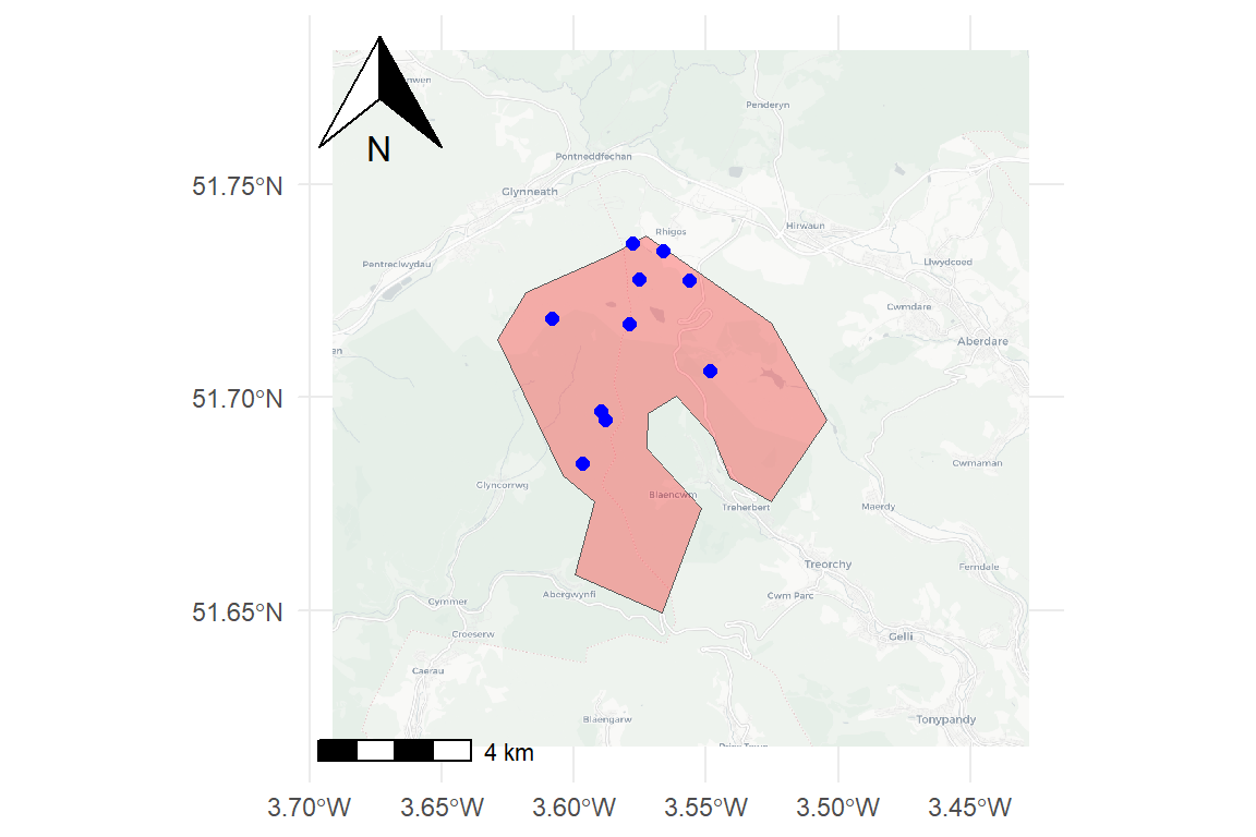
This function encapsulates the full workflow into a reusable tool. It takes a polygon, a minimum distance, and a desired number of points as inputs, then generates a spatial point dataset that satisfies the distance constraint. It also computes and attaches the nearest neighbour distance for each point.
# Function to generate random points within a polygon buffered by a minimum distance
# Attaches a dataframe of distances-between-points
#
# d = inherited distance (see rSSI documentation)
# n = number of points
# p = polygon
#
# E.g.
# spat <- Rpoints(d = 0.05, n = 50, p = poly1)
Rpoints <- function(d = 250, n = 10, p){

  stopifnot(inherits(p, "sf"))

  # Ensure projected CRS (meters)
  if (st_is_longlat(p)) {
    stop("Polygon must be projected (e.g., EPSG:27700)")
  }

  win <- as.owin(p)

  pts_ppp <- rSSI(r = d, n = n, win = win)

  pts <- st_as_sf(as.data.frame(pts_ppp), coords = c("x", "y"), crs = st_crs(p))

  dist_matrix <- st_distance(pts)

  nearest <- apply(dist_matrix, 1, function(v) min(v[v > 0]))

  pts |>
    mutate(min_dist_m = as.numeric(set_units(nearest, "m")))
}

# Example usage
spat <- Rpoints(d = 200, n = 30, p = poly)
head(spat)