Random forest and ensemble models

For this module, you’ll need the following packages:

sf
terra
geodata
randomForest
PresenceAbsence
AUC
RColorBrewer

Over the last three modules we’ve built and evaluated a GLM and a MaxEnt model for the mantled howler monkey. Both have strengths and weaknesses. The GLM is transparent and statistically rigorous but requires you to specify the functional form of every relationship. MaxEnt handles complex response shapes automatically but is a presence-background method with its own set of assumptions and a tendency to overfit if not carefully tuned.

In this module we add a third algorithm, random forest, and then do something more important than any individual model: we combine all three into an ensemble.

Why random forest?

Random forest is a machine learning algorithm that builds a large number of decision trees, each trained on a random subset of the data and a random subset of the predictor variables, then averages their predictions (Breiman 2001). The randomness is the point: individual trees are noisy but their average is stable. We’re basically applying the wisdom of crowds apporach to statistical models.

For species distribution modelling, random forest has several benefits. It handles nonlinear responses and interactions between predictors automatically, without us having to specify them. It doesn’t assume any particular distribution of the response variable. It produces a measure of variable importance as a by-product. And it generally performs well in comparative benchmarks across species and regions.

A random forest with 500 trees is not something you can read or explain the way you can explain a GLM coefficient, however. It’s a black box that produces predictions, not an ecological story. This is a genuine trade-off, and which side you prioritise depends on your goals.

Why ensemble models?

No single SDM algorithm is consistently the best across species, regions, and datasets. Different algorithms make different assumptions and fail in different ways. When we have multiple model predictions, the most robust approach is usually to combine them and average over model uncertainty rather than just using one algorithm.

This is the rationale behind ensemble modelling. Ensemble models consistently outperform individual algorithms in predictive accuracy benchmarks, and they give a natural measure of model uncertainty. Where all algorithms agree, confidence is high; where they disagree substantially, uncertainty is high (Araújo & New 2007). Conservation decisions made on the basis of SDMs are more defensible when they account for this uncertainty.

Load your data

load('data/region.RData')
load('data/module7_occdata.RData')
load('data/module10_sdm.RData')
load('data/module11_maxent.RData')
env_stack <- terra::rast('data/env_stack.tif')
bio_fut   <- terra::rast('data/bio_fut.tif')

# Load GLM and MaxEnt current and future predictions
pred_curr_glm    <- terra::rast('data/pred_current.tif')
pred_curr_maxent <- terra::rast('data/pred_maxent_curr.tif')
pred_fut_glm     <- terra::rast('data/pred_future.tif')
pred_fut_maxent  <- terra::rast('data/pred_maxent_fut.tif')

We’ll use the same training data and selected predictor variables as the previous two modules.

# Subset to selected predictors plus the response column
pred_sel <- c("bio10", "bio18", "bio15", "bio02", "bio13", "bio19")
rf_data <- howler_sdm[, c('occ', pred_sel)]

# Random forest requires the response to be a factor for classification
rf_data$occ <- as.factor(rf_data$occ)

table(rf_data$occ)

## 
##   0   1 
## 605 120

Fitting the random forest

randomForest() is the workhorse function. Key arguments:

ntree: number of trees to grow. More is generally better up to a point; 500–1000 is typical. We’ll use to reduce computational workload.
mtry: number of variables randomly sampled at each split. The default for classification is sqrt(number of predictors), which is usually reasonable.
importance = TRUE: calculate variable importance scores.

library(randomForest)

set.seed(42)

m_rf <- randomForest(
  occ ~ .,
  data       = rf_data,
  ntree      = 100,
  mtry       = floor(sqrt(length(pred_sel))),
  importance = TRUE
)

m_rf

## 
## Call:
##  randomForest(formula = occ ~ ., data = rf_data, ntree = 100,      mtry = floor(sqrt(length(pred_sel))), importance = TRUE) 
##                Type of random forest: classification
##                      Number of trees: 100
## No. of variables tried at each split: 2
## 
##         OOB estimate of  error rate: 19.31%
## Confusion matrix:
##     0  1 class.error
## 0 584 21  0.03471074
## 1 119  1  0.99166667

The OOB error rate (out-of-bag) in the output is an honest estimate of model error, computed on the training records that were left out of each individual tree (around 35%) by the bootstrap sampling process. It’s roughly equivalent to cross-validated error.

The confusion matrix in the output shows classification performance on the training data at a 0.5 threshold. Notice that random forest may classify more background points as “present” than absent. This is influenced by the class imbalance (5× more background than presence) and is worth keeping in mind when interpreting the map.

Variable importance

# Variable importance — two measures
importance(m_rf)

##              0          1 MeanDecreaseAccuracy MeanDecreaseGini
## bio10 7.678041 -11.254327             5.027019         14.69888
## bio18 7.431942  -9.818728             5.158520         12.31269
## bio15 7.072641  -8.567283             5.450444         12.89220
## bio02 5.348918 -10.069887             2.486253         13.11980
## bio13 7.621559  -8.354982             5.210630         11.55371
## bio19 8.422823  -8.956459             6.705005         11.73012

# Visualise
varImpPlot(m_rf, main = "Random forest variable importance",
           col = "tomato", pch = 19)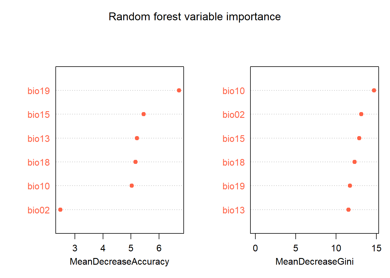

Two importance measures are shown:

MeanDecreaseAccuracy: how much model accuracy drops when each variable’s values are randomly permuted. Higher = more important. This is analogous to MaxEnt’s permutation importance.
MeanDecreaseGini: how much each variable reduces impurity in the trees. A secondary measure, less interpretable but sometimes useful.

Compare the importance ranking to those from the GLM (Module 9) and MaxEnt (Module 11). All three algorithms should broadly agree on which variables matter most. If they don’t, that’s worth investigating.

Cross-validation

Unlike MaxEnt, random forest doesn’t automatically produce spatially cross-validated predictions. We’ll use the same 5-fold cross-validation loop from Module 10 to keep evaluation consistent across all three algorithms.

set.seed(123)
k        <- 5
folds    <- sample(rep(1:k, length.out = nrow(rf_data)))
preds_rf <- numeric(nrow(rf_data))

for (i in 1:k) {
  train_rf <- rf_data[folds != i, ]
  test_rf  <- rf_data[folds == i, ]

  m_cv_rf  <- randomForest(
    occ ~ .,
    data  = train_rf,
    ntree = 500,
    mtry  = floor(sqrt(length(pred_sel)))
  )

  # predict() returns a matrix of class probabilities for classification RF
  preds_rf[folds == i] <- predict(m_cv_rf, newdata = test_rf, type = 'prob')[, '1']
}

Evaluating the random forest

library(AUC)
library(PresenceAbsence)

thresh_dat_rf <- data.frame(
  ID   = seq_len(nrow(howler_sdm)),
  obs  = howler_sdm$occ,
  pred = preds_rf
)

roc_rf <- AUC::roc(preds_rf, as.factor(howler_sdm$occ))
auc_rf <- AUC::auc(roc_rf)
cat("Random forest AUC:", auc_rf, "\n")

## Random forest AUC: 0.3418113

thresh_rf <- PresenceAbsence::optimal.thresholds(DATA = thresh_dat_rf)

## Warning in PresenceAbsence::optimal.thresholds(DATA = thresh_dat_rf): req.sens
## defaults to 0.85

## Warning in PresenceAbsence::optimal.thresholds(DATA = thresh_dat_rf): req.spec
## defaults to 0.85

## Warning in PresenceAbsence::optimal.thresholds(DATA = thresh_dat_rf): costs
## assumed to be equal

cmx_rf    <- PresenceAbsence::cmx(DATA = thresh_dat_rf, threshold = thresh_rf[3, 2])
sens_rf   <- PresenceAbsence::sensitivity(cmx_rf, st.dev = FALSE)
spec_rf   <- PresenceAbsence::specificity(cmx_rf, st.dev = FALSE)
tss_rf    <- sens_rf + spec_rf - 1
cat("Random forest TSS:", tss_rf, "\n")

## Random forest TSS: 0

Predictions across the landscape

# Build a data frame from the raster: one row per pixel
env_df    <- data.frame(crds(env_stack[[pred_sel]]), as.data.frame(env_stack[[pred_sel]]))
env_df_rf <- env_df[, pred_sel]   # random forest only needs the predictors, not coordinates

# Predict — type = 'prob' gives class probabilities
rf_probs <- predict(m_rf, newdata = env_df_rf, type = 'prob')

env_df$pred_rf <- rf_probs[, '1']   # probability of presence (class '1')

pred_curr_rf <- terra::rast(env_df[, c('x', 'y', 'pred_rf')],
                            type = 'xyz', crs = crs(env_stack))

plot(pred_curr_rf,
     main = "Random forest — predicted occurrence (current)",
     col  = rev(terrain.colors(100)))
plot(st_geometry(region), add = TRUE, border = "black", lwd = 1.2)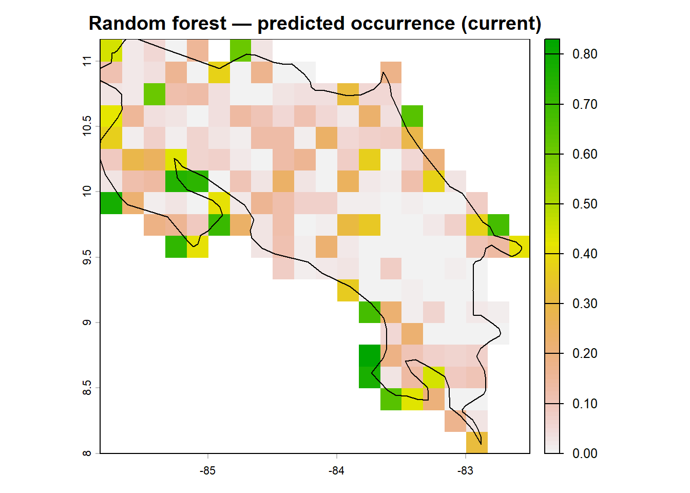

Now future climate:

fut_df    <- data.frame(crds(bio_fut[[pred_sel]]), as.data.frame(bio_fut[[pred_sel]]))
fut_rf    <- predict(m_rf, newdata = fut_df[, pred_sel], type = 'prob')
fut_df$pred_rf <- fut_rf[, '1']

pred_fut_rf <- terra::rast(fut_df[, c('x', 'y', 'pred_rf')],
                           type = 'xyz', crs = crs(env_stack))

Building the ensemble

Now to bring it all together. We combine the current-climate predictions from all three algorithms (GLM, MaxEnt, and random forest) into a single ensemble map. We’ll use a simple unweighted mean. This means that each algorithm gets equal weight, i.e., are equally valid or important. More sophisticated approaches weight algorithms by their cross-validated performance (Thuiller et al. 2009), but the simple mean is a reasonable starting point.

# Stack the three current predictions — they must share the same extent and resolution
# Resample if necessary to align grids
pred_maxent_resamp <- terra::resample(pred_curr_maxent, pred_curr_glm, method = 'bilinear')
pred_rf_resamp     <- terra::resample(pred_curr_rf,     pred_curr_glm, method = 'bilinear')

pred_stack_curr <- c(pred_curr_glm, pred_maxent_resamp, pred_rf_resamp)
names(pred_stack_curr) <- c('GLM', 'MaxEnt', 'RF')

# Ensemble mean
pred_ensemble_curr <- mean(pred_stack_curr, na.rm = TRUE)

# Ensemble uncertainty: standard deviation across algorithms
pred_ensemble_sd <- terra::app(pred_stack_curr, sd)

# Plot mean and uncertainty side by side
par(mfrow = c(1, 2))
plot(pred_ensemble_curr,
     main = "Ensemble mean — current climate",
     col  = rev(terrain.colors(100)), zlim = c(0, 1))
plot(st_geometry(region), add = TRUE, border = "black", lwd = 1.2)

plot(pred_ensemble_sd,
     main = "Ensemble uncertainty (SD)",
     col  = colorRampPalette(c("white", "steelblue", "navy"))(100))
plot(st_geometry(region), add = TRUE, border = "black", lwd = 1.2)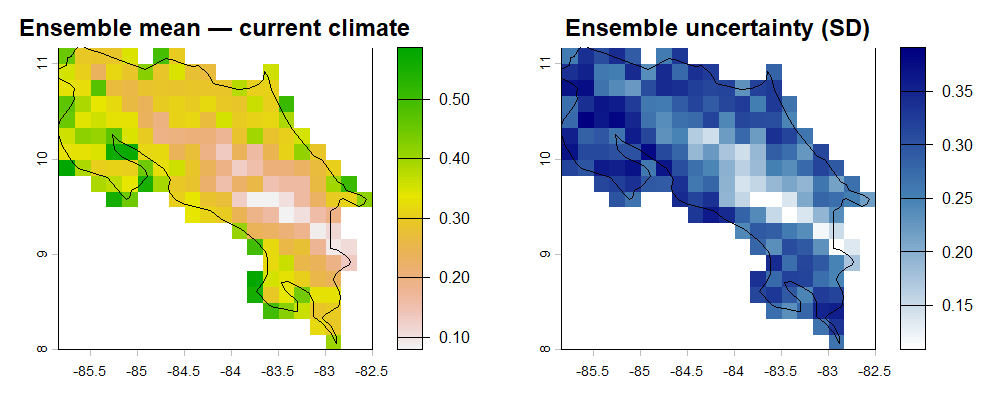

par(mfrow = c(1, 1))

The uncertainty map is arguably as important as the mean. Where the standard deviation is high, the three algorithms are disagreeing, i.e., they’re responding to different environmental signals or fitting different response shapes. These are exactly the areas where you should be most cautious about using the SDM for conservation decisions.

Where is uncertainty highest? Is it in areas of predicted high suitability, low suitability, or somewhere in between?

Ensemble under future climate

pred_maxent_fut_resamp <- terra::resample(pred_fut_maxent, pred_fut_glm, method = 'bilinear')
pred_rf_fut_resamp     <- terra::resample(pred_fut_rf,     pred_fut_glm, method = 'bilinear')

pred_stack_fut <- c(pred_fut_glm, pred_maxent_fut_resamp, pred_rf_fut_resamp)
names(pred_stack_fut) <- c('GLM', 'MaxEnt', 'RF')

pred_ensemble_fut <- mean(pred_stack_fut, na.rm = TRUE)
pred_ensemble_fut_sd <- terra::app(pred_stack_fut, sd)

# Four-panel summary
par(mfrow = c(2, 2))
plot(pred_ensemble_curr,    main = "Current — ensemble mean",   zlim = c(0, 1), col = rev(terrain.colors(100)))
plot(pred_ensemble_sd,      main = "Current — uncertainty",     col = colorRampPalette(c("white","steelblue","navy"))(100))
plot(pred_ensemble_fut,     main = "Future — ensemble mean",    zlim = c(0, 1), col = rev(terrain.colors(100)))
plot(pred_ensemble_fut_sd,  main = "Future — uncertainty",      col = colorRampPalette(c("white","steelblue","navy"))(100))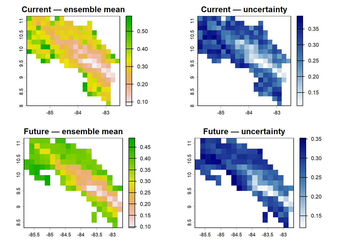

par(mfrow = c(1, 1))

A performance comparison across all three algorithms

Let’s put the performance metrics side by side so the full picture is clear.

comparison <- data.frame(
  Algorithm = c("GLM", "MaxEnt", "Random Forest"),
  AUC       = c(perf_summary$AUC, auc_mx, auc_rf),
  TSS       = c(perf_summary$TSS, tss_mx, tss_rf),
  D2_or_OOB = c(perf_summary$D2, NA, 1 - m_rf$err.rate[100, 'OOB'])
)

comparison

##       Algorithm       AUC       TSS  D2_or_OOB
## 1           GLM 0.5626377 0.1668733 0.02256085
## 2        MaxEnt 0.6030234 0.1670110         NA
## 3 Random Forest 0.3418113 0.0000000 0.80689655

No single algorithm “wins” across all metrics in every study. If random forest has the highest AUC but the GLM response curves make more biological sense, that’s worth noting. AUC measures discrimination, not ecological realism. If MaxEnt and random forest broadly agree on the distribution but the GLM disagrees, that’s worth investigating too.

The ensemble sidesteps the question of which algorithm is “best” by incorporating all three, producing a more robust prediction than any single model while making the uncertainty explicit.

Save your work

terra::writeRaster(pred_curr_rf,       'data/pred_rf_curr.tif',       overwrite = TRUE)
terra::writeRaster(pred_fut_rf,        'data/pred_rf_fut.tif',        overwrite = TRUE)
terra::writeRaster(pred_ensemble_curr, 'data/pred_ensemble_curr.tif', overwrite = TRUE)
terra::writeRaster(pred_ensemble_fut,  'data/pred_ensemble_fut.tif',  overwrite = TRUE)
terra::writeRaster(pred_ensemble_sd,   'data/pred_ensemble_sd.tif',   overwrite = TRUE)

save(m_rf, auc_rf, tss_rf, thresh_rf, comparison,
     file = 'data/module12_rf.RData')

Exercise

Build a weighted ensembleusing AUC as the weight for each algorithm. Multiply each prediction raster by its AUC, sum them, and divide by the sum of AUCs. How does the weighted ensemble map differ from the unweighted one? Where do the differences concentrate?
```
# Hint
w <- c(perf_summary$AUC, auc_mx, auc_rf)
pred_weighted <- (pred_stack_curr[[1]] * w[1] +
                  pred_stack_curr[[2]] * w[2] +
                  pred_stack_curr[[3]] * w[3]) / sum(w)
```
Produce a range change map by subtracting the current ensemble mean from the future ensemble mean. Cells with positive values are predicted gains; negative values are predicted losses. Where are the predicted losses for howler monkeys in Costa Rica under this climate scenario?
```
range_change <- pred_ensemble_fut - pred_ensemble_curr
plot(range_change,
     col  = colorRampPalette(c("tomato", "white", "steelblue"))(100),
     main = "Predicted range change (future - current)")
```
Look at the uncertainty map for the future predictions. Has uncertainty increased or decreased compared to the current climate map? What would increasing uncertainty under future climate imply for using these models in conservation planning?

Next steps

You may be looking at the plots and metrics and wondering about the accuracy and utility of these models. That’s a very common situation in SDMs wherein the algorithm is fine, but the ecological signal is incomplete. If key drivers like human pressure or habitat degradation aren’t in the predictors then even the best model will struggle.

Here are some next-step exercises that will might produce a noticeable improvement:

Add human impact / accessibility layers. A big omission in many SDMs is that species are often limited by humans more than climate. You could therefore look to add potentially important metrics like

Core habitat constraints (e.g., forest cover, tree canopy density)
Disturbance / human pressure (e.g., distance to roads, human footprint index, artificial light at night)
Fragmentation metrics (e.g., patch size, connectivity index)

Correct for sampling bias in presence data. Occurrence data are rarely evenly sampled in space, as we’ve discussed. Create a bias surface (e.g., kernel density of all records or sampling effort proxies) and use it to direct background sampling in MaxEnt, or weighted sampling in RF / GLM.
Incorporate bias into your ensemble. Right now, all models are treated as equally good—even if they’re not.Try weighting models by AUC, TSS, or some other metric ad compare with the unweighted ensemble.

References

Araújo, M.B. & New, M. (2007). Ensemble forecasting of species distributions. Trends in Ecology and Evolution, 22, 42–47.

Breiman, L. (2001). Random forests. Machine Learning, 45, 5–32.

Thuiller, W., Lafourcade, B., Engler, R. & Araújo, M.B. (2009). BIOMOD — a platform for ensemble forecasting of species distributions. Ecography, 32, 369–373.

← Previous