MaxEnt — maximum entropy modelling

For this module, you’ll need the following packages:

• sf
• terra
• geodata
• ENMeval
• PresenceAbsence
• AUC

You’ll also need Java installed on your system, as MaxEnt runs on the Java Virtual Machine. ENMeval will prompt you if it’s missing.

In the last two modules we built a logistic regression SDM, evaluated it, and projected it under current and future climate. The GLM is a solid, interpretable starting point but it makes assumptions that may not always hold. It requires you to manually specify the shape of species-environment relationships (linear? quadratic?), it handles interactions between variables poorly unless you explicitly include them, and it can struggle when relationships are genuinely complex or nonlinear.

MaxEnt takes a different approach entirely. Rather than fitting a regression, it finds the probability distribution of species occurrence that is as spread out (has maximum entropy) as possible while still matching the observed environmental conditions at occurrence points. The intuition is that MaxEnt doesn’t assume more than it has to. This makes it well suited to presence-background data, where we have records of where a species was found but no reliable information about where it wasn’t.

MaxEnt has been the dominant SDM algorithm in ecology for some time (Phillips et al. 2006) and is still among the best-performing algorithms across comparative studies. If you read SDM papers, you will encounter it constantly.

A note on overfitting and regularisation

MaxEnt’s default settings have a well-documented problem: they tend to produce overfitted models. The algorithm can fit very complex, wiggly response surfaces that track the training data closely but generalise poorly to new locations or time periods. This is controlled by a regularisation multiplier where higher values produce smoother, more generalised predictions; lower values allow more complex fits.

The default regularisation in MaxEnt (β = 1) was chosen for a general-purpose setting and is often too low for real datasets, especially when occurrence records are few or spatially biased. Using it uncritically is one of the most common methodological errors in published SDM work (Warren & Seifert 2011, Merow et al. 2013).

We’ll use the ENMeval package, which automates the selection of the best regularisation value using cross-validation. It also lets us test different feature types (the shapes of response functions MaxEnt can fit), which is the other main tuning decision.

Load your data

load('data/region.RData')
load('data/module7_occdata.RData')
load('data/module10_sdm.RData')
env_stack <- terra::rast('data/env_stack.tif')
env_vars <- read.csv("data/env_vars.csv")

MaxEnt needs presence coordinates and background coordinates as separate data frames, plus the raster stack as a SpatRaster.

# Presence coordinates
occ_coords <- howler_sdm[howler_sdm$occ == 1, c('x', 'y')]

# Background coordinates
bg_coords  <- howler_sdm[howler_sdm$occ == 0, c('x', 'y')]

nrow(occ_coords)

## [1] 120

nrow(bg_coords)

## [1] 605

We’ll use the same selected predictors from Module 9 to keep the comparison to the GLM fair.

# Subset the raster stack to selected predictors only
pred_sel <- c("bio10", "bio18", "bio15", "bio02", "bio13", "bio19")
env_sel <- env_stack[[pred_sel]]
env_sel

## class       : SpatRaster 
## size        : 19, 20, 6  (nrow, ncol, nlyr)
## resolution  : 0.1666667, 0.1666667  (x, y)
## extent      : -85.83333, -82.5, 8, 11.16667  (xmin, xmax, ymin, ymax)
## coord. ref. : lon/lat WGS 84 (EPSG:4326) 
## source      : env_stack.tif 
## names       :    bio10, bio18,    bio15,     bio02, bio13, bio19 
## min values  : 12.42479,   210, 23.76402,  6.975149,   316,   129 
## max values  : 28.77827,   917, 97.51337, 11.785084,   642,  1376

Tuning MaxEnt with ENMeval

ENMeval fits MaxEnt across a grid of regularisation multipliers and feature type combinations, evaluating each with spatial block cross-validation. Spatial block cross-validation is used instead of random cross-validation for SDMs because it is more applicable to predicting to new geographic areas (Valavi et al. 2019).

Feature types define the shapes of response functions MaxEnt can use:

• L (linear): straight-line responses
• Q (quadratic): curved, hump-shaped responses — analogous to the I(x^2) terms in our GLM
• P (product): interactions between pairs of variables
• H (hinge): piecewise linear responses that can change slope at a threshold
• T (threshold): step functions

We’ll test combinations of L, Q, and H across a range of regularisation multipliers from 0.5 to 4. This produces a grid of candidate models that we can evaluate and select from.

set.seed(42)

enmeval_results <- ENMevaluate(
  occs      = occ_coords,
  envs      = env_sel,
  bg        = bg_coords,
  algorithm = 'maxnet',        # maxnet is the R-native MaxEnt implementation
  partitions = 'block',        # spatial block cross-validation
  tune.args = list(
    fc = c('L', 'LQ', 'LQH'),  # feature type combinations to test
    rm = seq(0.5, 4, by = 0.5) # regularisation multipliers to test
  )
)

## Package ecospat is not installed, so Continuous Boyce Index (CBI) cannot be calculated.

## *** Running initial checks... ***

## * Clamping predictor variable rasters...

## * Model evaluations with spatial block (4-fold) cross validation and lat_lon orientation...

## 
## *** Running ENMeval v2.0.5 with maxnet from maxnet package v0.1.4 ***

##   |                                                                              |                                                                      |   0%  |                                                                              |===                                                                   |   4%  |                                                                              |======                                                                |   8%  |                                                                              |=========                                                             |  12%  |                                                                              |============                                                          |  17%  |                                                                              |===============                                                       |  21%  |                                                                              |==================                                                    |  25%  |                                                                              |====================                                                  |  29%  |                                                                              |=======================                                               |  33%  |                                                                              |==========================                                            |  38%  |                                                                              |=============================                                         |  42%  |                                                                              |================================                                      |  46%  |                                                                              |===================================                                   |  50%  |                                                                              |======================================                                |  54%  |                                                                              |=========================================                             |  58%  |                                                                              |============================================                          |  62%  |                                                                              |===============================================                       |  67%  |                                                                              |==================================================                    |  71%  |                                                                              |====================================================                  |  75%  |                                                                              |=======================================================               |  79%  |                                                                              |==========================================================            |  83%  |                                                                              |=============================================================         |  88%  |                                                                              |================================================================      |  92%  |                                                                              |===================================================================   |  96%  |                                                                              |======================================================================| 100%

## Making model prediction rasters...

## ENMevaluate completed in 0 minutes 47.6 seconds.

enmeval_results

## An object of class:  ENMevaluation 
##  occurrence/background points:  120 / 605 
##  partition method:  block 
##  partition settings:  orientation = lat_lon 
##  clamp:  left: bio10, bio18, bio15, bio02, bio13, bio19
##          right: bio10, bio18, bio15, bio02, bio13, bio19 
##  categoricals:   
##  algorithm:  maxnet 
##  tune settings:  fc: L,LQ,LQH
##                  rm: 0.5,1.0,1.5,2.0,2.5,3.0,3.5,4.0 
##  overlap:  TRUE 
## Refer to ?ENMevaluation for information on slots.

This may take a minute or two as it’s fitting many models, not just one. The output summarises performance across the full tuning grid.

Selecting the best model

We select the model with the lowest AICc (AIC corrected for small sample sizes) across the tuning grid. AICc balances model fit against complexity, penalising models that use more parameters to achieve only small improvements in fit.

# Model results table, sorted by AICc
results_tab <- eval.results(enmeval_results)
results_tab[order(results_tab$AICc), ]

##     fc  rm     tune.args auc.train cbi.train auc.diff.avg auc.diff.sd
## 22   L 4.0     fc.L_rm.4 0.6030234        NA   0.09801208  0.05832281
## 19   L 3.5   fc.L_rm.3.5 0.6034780        NA   0.09553865  0.05816894
## 16   L 3.0     fc.L_rm.3 0.6039050        NA   0.09315217  0.05853376
## 13   L 2.5   fc.L_rm.2.5 0.6043733        NA   0.08783816  0.05203932
## 11  LQ 2.0    fc.LQ_rm.2 0.6118113        NA   0.09425845  0.03303337
## 12 LQH 2.0   fc.LQH_rm.2 0.6118113        NA   0.09425845  0.03303337
## 10   L 2.0     fc.L_rm.2 0.6045799        NA   0.08369807  0.04432787
## 14  LQ 2.5  fc.LQ_rm.2.5 0.6119490        NA   0.09468357  0.03438502
## 15 LQH 2.5 fc.LQH_rm.2.5 0.6119490        NA   0.09468357  0.03438502
## 18 LQH 3.0   fc.LQH_rm.3 0.6109298        NA   0.09573188  0.04171801
## 17  LQ 3.0    fc.LQ_rm.3 0.6109298        NA   0.09573188  0.04171801
## 20  LQ 3.5  fc.LQ_rm.3.5 0.6103099        NA   0.09819082  0.04691824
## 21 LQH 3.5 fc.LQH_rm.3.5 0.6103099        NA   0.09819082  0.04691824
## 23  LQ 4.0    fc.LQ_rm.4 0.6101860        NA   0.09949034  0.05331123
## 24 LQH 4.0   fc.LQH_rm.4 0.6101860        NA   0.09949034  0.05331123
## 4    L 1.0     fc.L_rm.1 0.6046350        NA   0.06835990  0.04781736
## 7    L 1.5   fc.L_rm.1.5 0.6046763        NA   0.07671739  0.04176154
## 8   LQ 1.5  fc.LQ_rm.1.5 0.6125275        NA   0.09221014  0.03530768
## 1    L 0.5   fc.L_rm.0.5 0.6045248        NA   0.06860628  0.04519654
## 5   LQ 1.0    fc.LQ_rm.1 0.6165909        NA   0.08326329  0.03954120
## 9  LQH 1.5 fc.LQH_rm.1.5 0.6128306        NA   0.07616184  0.05712824
## 2   LQ 0.5  fc.LQ_rm.0.5 0.6222934        NA   0.04215217  0.05504481
## 6  LQH 1.0   fc.LQH_rm.1 0.6192080        NA   0.06003140  0.05293013
## 3  LQH 0.5 fc.LQH_rm.0.5 0.6368664        NA   0.07331643  0.04063869
##    auc.val.avg auc.val.sd cbi.val.avg cbi.val.sd or.10p.avg  or.10p.sd
## 22   0.5904275 0.10599337          NA         NA  0.1000000 0.08164966
## 19   0.5908478 0.10431172          NA         NA  0.1083333 0.09179284
## 16   0.5914565 0.10227222          NA         NA  0.1083333 0.09179284
## 13   0.5936304 0.09663695          NA         NA  0.1000000 0.08164966
## 11   0.6021232 0.09615553          NA         NA  0.1250000 0.09953596
## 12   0.6021232 0.09615553          NA         NA  0.1250000 0.09953596
## 10   0.5985290 0.09016591          NA         NA  0.1000000 0.08164966
## 14   0.5958768 0.09643635          NA         NA  0.1166667 0.08819171
## 15   0.5958768 0.09643635          NA         NA  0.1166667 0.08819171
## 18   0.5912681 0.09842335          NA         NA  0.1250000 0.09953596
## 17   0.5912681 0.09842335          NA         NA  0.1250000 0.09953596
## 20   0.5885145 0.10173466          NA         NA  0.1250000 0.09953596
## 21   0.5885145 0.10173466          NA         NA  0.1250000 0.09953596
## 23   0.5850507 0.10466418          NA         NA  0.1083333 0.07876359
## 24   0.5850507 0.10466418          NA         NA  0.1083333 0.07876359
## 4    0.6085580 0.07654977          NA         NA  0.1083333 0.07876359
## 7    0.6031377 0.08262090          NA         NA  0.1000000 0.08164966
## 8    0.6103406 0.09452707          NA         NA  0.1333333 0.08606630
## 1    0.6172971 0.07266968          NA         NA  0.1083333 0.07391186
## 5    0.6154710 0.08781593          NA         NA  0.1166667 0.07934920
## 9    0.6181812 0.08699869          NA         NA  0.1000000 0.05443311
## 2    0.6300797 0.06300490          NA         NA  0.1000000 0.07200823
## 6    0.6323551 0.06804289          NA         NA  0.1000000 0.07200823
## 3    0.6227754 0.05264982          NA         NA  0.1666667 0.07200823
##     or.mtp.avg  or.mtp.sd     AICc  delta.AICc        w.AIC ncoef
## 22 0.025000000 0.05000000 1260.015  0.00000000 1.580819e-01     3
## 19 0.025000000 0.05000000 1260.057  0.04207120 1.547913e-01     3
## 16 0.025000000 0.05000000 1260.104  0.08876211 1.512195e-01     3
## 13 0.008333333 0.01666667 1260.157  0.14223995 1.472296e-01     3
## 11 0.016666667 0.03333333 1261.903  1.88773026 6.151297e-02     4
## 12 0.016666667 0.03333333 1261.903  1.88773026 6.151297e-02     4
## 10 0.008333333 0.01666667 1262.293  2.27801199 5.060788e-02     4
## 14 0.025000000 0.05000000 1264.061  4.04578800 2.090983e-02     5
## 15 0.025000000 0.05000000 1264.061  4.04578800 2.090983e-02     5
## 18 0.025000000 0.05000000 1264.107  4.09241915 2.042794e-02     5
## 17 0.025000000 0.05000000 1264.107  4.09241915 2.042794e-02     5
## 20 0.025000000 0.05000000 1264.179  4.16426713 1.970711e-02     5
## 21 0.025000000 0.05000000 1264.179  4.16426713 1.970711e-02     5
## 23 0.025000000 0.05000000 1264.275  4.25991692 1.878680e-02     5
## 24 0.025000000 0.05000000 1264.275  4.25991692 1.878680e-02     5
## 4  0.008333333 0.01666667 1264.368  4.35321288 1.793056e-02     5
## 7  0.008333333 0.01666667 1264.404  4.38897914 1.761276e-02     5
## 8  0.016666667 0.03333333 1266.339  6.32432625 6.692250e-03     6
## 1  0.008333333 0.01666667 1266.546  6.53148190 6.033771e-03     6
## 5  0.008333333 0.01666667 1267.978  7.96339148 2.948856e-03     7
## 9  0.025000000 0.05000000 1268.585  8.57045894 2.176861e-03     7
## 2  0.000000000 0.00000000 1268.769  8.75445586 1.985529e-03     8
## 6  0.025000000 0.05000000 1294.587 34.57206287 4.916478e-09    18
## 3  0.033333333 0.03849002 1339.705 79.69044521 7.840104e-19    33

# The best model by AICc
best_settings <- results_tab[which.min(results_tab$AICc), ]
best_settings

##    fc rm tune.args auc.train cbi.train auc.diff.avg auc.diff.sd auc.val.avg
## 22  L  4 fc.L_rm.4 0.6030234        NA   0.09801208  0.05832281   0.5904275
##    auc.val.sd cbi.val.avg cbi.val.sd or.10p.avg  or.10p.sd or.mtp.avg or.mtp.sd
## 22  0.1059934          NA         NA        0.1 0.08164966      0.025      0.05
##        AICc delta.AICc     w.AIC ncoef
## 22 1260.015          0 0.1580819     3

cat("Best feature class:", best_settings$fc, "\n")

## Best feature class: L

cat("Best regularisation:", best_settings$rm, "\n")

## Best regularisation: 4

Take note of the selected regularisation multiplier. Is it close to the default of 1, or substantially different? A higher value suggests the data support a simpler, more generalised model than the default would produce.

# Extract the best fitted model object
m_maxent <- eval.models(enmeval_results)[[best_settings$tune.args]]

Response curves

MaxEnt’s response curves show how predicted suitability changes along each predictor while others are held at their mean. This is the same concept as the partial response plots in Module 10.

# Response curves for each selected predictor
plot(m_maxent, vars = pred_sel, 
     type = 'cloglog',
     ylab = 'Predicted suitability',
     col = 'tomato', 
     lwd = 2)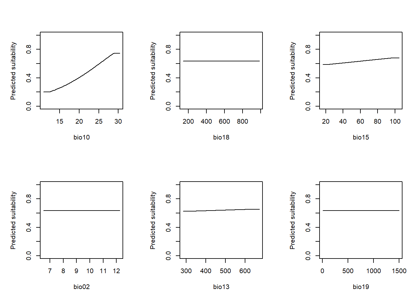

The cloglog transformation converts MaxEnt’s raw output to an approximate occurrence probability on a 0–1 scale that is comparable to the probabilities produced by the GLM. Compare the shapes here to the partial response curves from Module 10. Do the two algorithms agree on the direction and shape of relationships?

Variable importance

One advantage of MaxEnt over a GLM is that it provides a measure of variable contribution directly. Two metrics are available:

• Percent contribution: how much each variable contributed to the final model during training
• Permutation importance: how much model performance drops when each variable’s values are randomly shuffled

# Variable importance
# Ensure predictor names match model
env_sel <- env_stack[[pred_sel]]

# Baseline prediction
base_pred <- terra::predict(env_sel, 
                            m_maxent, type = "cloglog", 
                            na.rm = TRUE)
base_vals <- values(base_pred)

#Permutation importance
perm_imp <- sapply(names(env_sel), function(v) {
  perm_env <- env_sel
  perm_env[[v]] <- sample(perm_env[[v]])
  perm_pred <- terra::predict(perm_env, #
                              m_maxent, 
                              type = "cloglog", 
                              na.rm = TRUE)
  perm_vals <- values(perm_pred)
  cor(base_vals, perm_vals, use = "complete.obs")   # importance = loss of agreement with baseline
})

perm_imp <- 1 - perm_imp  # convert to "importance"

# Contribution proxy (maxnet doesn't store training contribution cleanly)
coef_vals <- m_maxent$betas
coef_names <- names(coef_vals)

# Match only environmental variables (ignore regularisation terms)
contrib_proxy <- sapply(names(env_sel), function(v) {
  sum(abs(coef_vals[grepl(v, coef_names)]), na.rm = TRUE)
})

contrib_proxy <- contrib_proxy / sum(contrib_proxy)

# Final table
var_imp <- data.frame(  
  variable = names(env_sel),
  permutation_importance = perm_imp,
  contribution_proxy = contrib_proxy
)

var_imp <- var_imp[order(var_imp$permutation_importance, 
                         decreasing = TRUE), ]
var_imp

##       variable permutation_importance contribution_proxy
## bio10    bio10           0.5403022948        0.968346293
## bio15    bio15           0.0154198557        0.029544482
## bio13    bio13           0.0009704628        0.002109225
## bio18    bio18           0.0000000000        0.000000000
## bio02    bio02           0.0000000000        0.000000000
## bio19    bio19           0.0000000000        0.000000000

Do the most important variables match your expectations from Module 8? Do they agree with the variables that ended up in the stepwise GLM?

Predictions and evaluation

Let’s generate predictions and evaluate them using the same framework as Module 10, so the comparison to the GLM is direct.

# Predict across the current climate raster
pred_maxent_curr <- terra::predict(env_sel, m_maxent, 
                                   type = 'cloglog',
                                   na.rm = TRUE)

plot(pred_maxent_curr,
     main = "MaxEnt — predicted suitability (current climate)",
     col  = rev(terrain.colors(100)))
plot(st_geometry(region), add = TRUE, 
     border = "black", 
     lwd = 1.2)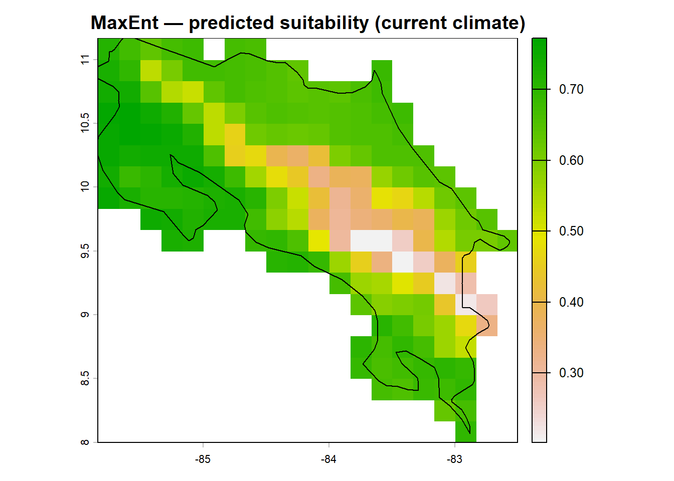

Now evaluate with cross-validated predictions. We’ll extract the cross-validated predictions from the ENMeval results object. These were already computed during the tuning step, so no extra computation is needed.

library(AUC)
library(PresenceAbsence)

# Cross-validated predictions are stored in the results object
# We need to reconstruct them from the evaluation partition predictions
best_i <- which.min(eval.results(enmeval_results)$AICc)
cv_preds_maxent <- eval.predictions(enmeval_results)[[best_i]]

# Extract the values at occurrence and background points
occ_preds <- cv_preds_maxent[eval.occs.grp(enmeval_results) > 0]

## Warning in Ops.factor(eval.occs.grp(enmeval_results), 0): '>' not meaningful
## for factors

bg_preds  <- cv_preds_maxent

# Build evaluation data frame
thresh_dat_mx <- data.frame(
  ID   = seq_len(nrow(howler_sdm)),
  obs  = howler_sdm$occ,
  pred = c(
    terra::extract(cv_preds_maxent, vect(
      st_as_sf(occ_coords, coords = c('x','y'), crs = 4326)
    ))[, 2],
    terra::extract(cv_preds_maxent, vect(
      st_as_sf(bg_coords, coords = c('x','y'), crs = 4326)
    ))[, 2]
  )
)
thresh_dat_mx <- na.omit(thresh_dat_mx)

# AUC
roc_mx <- AUC::roc(thresh_dat_mx$pred, 
                   as.factor(thresh_dat_mx$obs))
auc_mx <- AUC::auc(roc_mx)
cat("MaxEnt AUC:", auc_mx, "\n")

## MaxEnt AUC: 0.6030234

# Threshold and TSS
thresh_mx <- PresenceAbsence::optimal.thresholds(DATA = thresh_dat_mx)

## Warning in PresenceAbsence::optimal.thresholds(DATA = thresh_dat_mx): req.sens
## defaults to 0.85

## Warning in PresenceAbsence::optimal.thresholds(DATA = thresh_dat_mx): req.spec
## defaults to 0.85

## Warning in PresenceAbsence::optimal.thresholds(DATA = thresh_dat_mx): costs
## assumed to be equal

cmx_mx    <- PresenceAbsence::cmx(DATA = thresh_dat_mx, 
                                  threshold = thresh_mx[3, 2])
sens_mx   <- PresenceAbsence::sensitivity(cmx_mx, st.dev = FALSE)
spec_mx   <- PresenceAbsence::specificity(cmx_mx, st.dev = FALSE)
tss_mx    <- sens_mx + spec_mx - 1

cat("MaxEnt TSS:", tss_mx, "\n")

## MaxEnt TSS: 0.167011

How does MaxEnt perform compared to the GLM from Module 10? Remember that a better AUC doesn’t necessarily mean a better ecological model. A more complex algorithm can overfit to spatial patterns in the training data rather than capturing real environmental responses.

Predicting under future climate

bio_fut <- terra::rast('data/bio_fut.tif')

# Subset future climate to selected predictors
bio_fut_sel <- bio_fut[[pred_sel]]

pred_maxent_fut <- terra::predict(bio_fut_sel, m_maxent, 
                                  type = 'cloglog',
                                  na.rm = TRUE)

par(mfrow = c(1, 2))
plot(pred_maxent_curr, main = "Current climate",        
     zlim = c(0, 1),
     col = rev(terrain.colors(100)))
plot(pred_maxent_fut,  main = "Future climate (2041–60)", 
     zlim = c(0, 1),
     col = rev(terrain.colors(100)))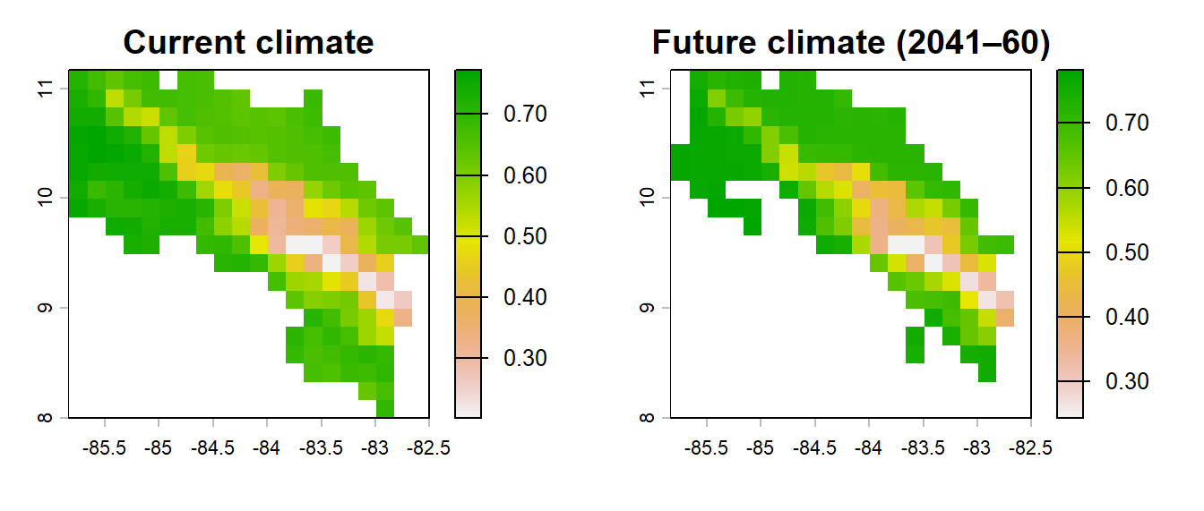

par(mfrow = c(1, 1))

Save your work

terra::writeRaster(pred_maxent_curr, 'data/pred_maxent_curr.tif', overwrite = TRUE)
terra::writeRaster(pred_maxent_fut,  'data/pred_maxent_fut.tif',  overwrite = TRUE)

save(m_maxent, best_settings, auc_mx, tss_mx, thresh_mx,
     file = 'data/module11_maxent.RData')

Exercise

1. Re-run ENMevaluate() with a wider regularisation range (e.g. rm = seq(0.5, 6, by = 0.5)). Does the selected regularisation multiplier change? Plot the AICc values across the full tuning grid to see how sensitive the selection is.

2. Compare the MaxEnt response curve for p1 to the partial response curve from the GLM (Module 10). Are the shapes similar? If they differ substantially, what might that tell you about the assumptions each algorithm is making?

3. Look at the variable importance table. Does the ranking from permutation.importance match the ranking from the univariate AIC selection in Module 9? What does disagreement between these rankings suggest?

References

Merow, C., Smith, M.J. & Silander, J.A. (2013). A practical guide to MaxEnt for modeling species’ distributions: what it does, and why inputs and settings matter. Ecography, 36, 1058–1069.
Phillips, S.J., Anderson, R.P. & Schapire, R.E. (2006). Maximum entropy modeling of species geographic distributions. Ecological Modelling, 190, 231–259.
Valavi, R., Elith, J., Lahoz-Monfort, J.J. & Guillera-Arroita, G. (2019). blockCV: an R package for generating spatially or environmentally separated folds for k-fold cross-validation of species distribution models. Methods in Ecology and Evolution, 10, 225–232.
Warren, D.L. & Seifert, S.N. (2011). Ecological niche modeling in Maxent: the importance of model complexity and the performance of model selection criteria. Ecological Applications, 21, 335–342.