Opening and exploring spatial data in R
For this module, you’ll need the following packages:
sfrgbif
So far, we’ve talked about what spatial data is and why it matters. Now comes the hands-on part — actually getting it into R and having a look around.
When you load spatial data into R, it doesn’t appear as a neat table like a spreadsheet. Instead, it’s stored in special objects that keep track of both the data (species names, counts, measurements) and the geometry (where those things are). Think of it as a spreadsheet with a built-in map attached — which is essentially what it is.
If we had data from a primate survey, it might look like this:
| Site ID | Species seen | Temperature | Location |
|---|---|---|---|
| 1 | Yes | 27.4°C | (x₁, y₁) |
| 2 | No | 24.1°C | (x₂, y₂) |
The Location column isn’t plain text — it’s
geometry. It contains the coordinates that allow R to map and spatially
analyse those data. This is the fundamental structure of a
simple features object, which is what the
sf package works with (Pebesma 2018). The “simple features”
standard is an international specification for how geographic vector
data should be represented, and sf is its R
implementation.
Where does our species data come from?
We’ll use the Global Biodiversity Information
Facility (GBIF) — a huge open-access database of biodiversity
observations compiled from museum collections, citizen science
platforms, research surveys, and automated monitoring. It currently
holds over 2 billion occurrence records and is one of the primary data
sources in contemporary macroecology and conservation biology
(Chamberlain & Boettiger 2017). The rgbif package lets
us query it directly from R, which means we can pull real data, from a
real database, and work with it immediately.
That said, GBIF data comes with important caveats. Records are contributed by many sources with wildly varying standards of accuracy and completeness. Coordinates can be imprecise, duplicated, or wrong. Sampling effort is deeply uneven — well-studied areas near roads and research stations are heavily over-represented. We will deal with all of this carefully in Module 7. For now, we load and explore.
Loading packages
# install.packages(c("sf", "rgbif"))  # only run once
library(sf)
library(rgbif)
Downloading howler monkey records
Let’s download occurrence records for the mantled howler monkey (Alouatta palliata). We’ll keep the download modest to start (just 300 records) to keep things quick. We’ll work with a fuller, geographically filtered dataset from Module 4 onwards.
howler <- occ_search(
  scientificName = "Alouatta palliata",
  limit = 300,
  hasCoordinate = TRUE  # only return records with usable coordinates
)
Turning it into spatial data
Right now howler$data is a plain data frame — rows and
columns, nothing spatial. We tell R which columns contain the
coordinates and what coordinate system they use. We’ll discuss
coordinate systems properly in Module 3; for now,
crs = 4326 refers to WGS84, the standard global system used
by GPS receivers and GBIF.
howler_sf <- st_as_sf(
  howler$data,
  coords = c("decimalLongitude", "decimalLatitude"),
  crs = 4326
)

howler_sf
## Simple feature collection with 300 features and 105 fields
## Geometry type: POINT
## Dimension: XY
## Bounding box: xmin: -94.50629 ymin: -3.743768 xmax: -77.36822 ymax: 18.37124
## Geodetic CRS: WGS 84
## # A tibble: 300 × 106
## key scientificName issues datasetKey publishingOrgKey installationKey
## * <chr> <chr> <chr> <chr> <chr> <chr>
## 1 5938036987 Alouatta palli… cdc,c… 50c9509d-… 28eb1a3f-1c15-4… 997448a8-f762-…
## 2 5938118541 Alouatta palli… cdc,c… 50c9509d-… 28eb1a3f-1c15-4… 997448a8-f762-…
## 3 5938193003 Alouatta palli… cdc,c… 50c9509d-… 28eb1a3f-1c15-4… 997448a8-f762-…
## 4 5938235647 Alouatta palli… cdc,c… 50c9509d-… 28eb1a3f-1c15-4… 997448a8-f762-…
## 5 5938269984 Alouatta palli… cdc,c… 50c9509d-… 28eb1a3f-1c15-4… 997448a8-f762-…
## 6 5938276988 Alouatta palli… cdc,c… 50c9509d-… 28eb1a3f-1c15-4… 997448a8-f762-…
## 7 5938279221 Alouatta palli… cdc,c… 50c9509d-… 28eb1a3f-1c15-4… 997448a8-f762-…
## 8 5938302462 Alouatta palli… cdc,c… 50c9509d-… 28eb1a3f-1c15-4… 997448a8-f762-…
## 9 5938375614 Alouatta palli… cdc,c… 50c9509d-… 28eb1a3f-1c15-4… 997448a8-f762-…
## 10 5938407216 Alouatta palli… cdc,c… 50c9509d-… 28eb1a3f-1c15-4… 997448a8-f762-…
## # ℹ 290 more rows
## # ℹ 100 more variables: hostingOrganizationKey <chr>, publishingCountry <chr>,
## # protocol <chr>, lastCrawled <chr>, lastParsed <chr>, crawlId <int>,
## # basisOfRecord <chr>, occurrenceStatus <chr>, taxonKey <int>,
## # kingdomKey <int>, phylumKey <int>, classKey <int>, orderKey <int>,
## # familyKey <int>, genusKey <int>, speciesKey <int>, acceptedTaxonKey <int>,
## # acceptedScientificName <chr>, kingdom <chr>, phylum <chr>, order <chr>, …You’ll see rows of observations, columns like country,
stateProvince, and eventDate, and, crucially,
a geometry column of type POINT. That geometry column is
what makes this a spatial object. Everything else in the sf
package flows from it.
summary(howler_sf)## key scientificName issues datasetKey
## Length:300 Length:300 Length:300 Length:300
## Class :character Class :character Class :character Class :character
## Mode :character Mode :character Mode :character Mode :character
##
##
##
##
## publishingOrgKey installationKey hostingOrganizationKey
## Length:300 Length:300 Length:300
## Class :character Class :character Class :character
## Mode :character Mode :character Mode :character
##
##
##
##
## publishingCountry protocol lastCrawled lastParsed
## Length:300 Length:300 Length:300 Length:300
## Class :character Class :character Class :character Class :character
## Mode :character Mode :character Mode :character Mode :character
##
##
##
##
## crawlId basisOfRecord occurrenceStatus taxonKey
## Min. :196.0 Length:300 Length:300 Min. :2436649
## 1st Qu.:594.0 Class :character Class :character 1st Qu.:2436649
## Median :594.0 Mode :character Mode :character Median :2436649
## Mean :579.2 Mean :2830703
## 3rd Qu.:594.0 3rd Qu.:2436649
## Max. :594.0 Max. :7342629
##
## kingdomKey phylumKey classKey orderKey familyKey
## Min. :1 Min. :44 Min. :359 Min. :798 Min. :3239607
## 1st Qu.:1 1st Qu.:44 1st Qu.:359 1st Qu.:798 1st Qu.:3239607
## Median :1 Median :44 Median :359 Median :798 Median :3239607
## Mean :1 Mean :44 Mean :359 Mean :798 Mean :3239607
## 3rd Qu.:1 3rd Qu.:44 3rd Qu.:359 3rd Qu.:798 3rd Qu.:3239607
## Max. :1 Max. :44 Max. :359 Max. :798 Max. :3239607
##
## genusKey speciesKey acceptedTaxonKey acceptedScientificName
## Min. :2436647 Min. :2436649 Min. :2436649 Length:300
## 1st Qu.:2436647 1st Qu.:2436649 1st Qu.:2436649 Class :character
## Median :2436647 Median :2436649 Median :2436649 Mode :character
## Mean :2436647 Mean :2436649 Mean :2830703
## 3rd Qu.:2436647 3rd Qu.:2436649 3rd Qu.:2436649
## Max. :2436647 Max. :2436649 Max. :7342629
##
## kingdom phylum order family
## Length:300 Length:300 Length:300 Length:300
## Class :character Class :character Class :character Class :character
## Mode :character Mode :character Mode :character Mode :character
##
##
##
##
## genus species genericName specificEpithet
## Length:300 Length:300 Length:300 Length:300
## Class :character Class :character Class :character Class :character
## Mode :character Mode :character Mode :character Mode :character
##
##
##
##
## taxonRank taxonomicStatus iucnRedListCategory dateIdentified
## Length:300 Length:300 Length:300 Length:300
## Class :character Class :character Class :character Class :character
## Mode :character Mode :character Mode :character Mode :character
##
##
##
##
## coordinateUncertaintyInMeters continent stateProvince
## Min. : 1.0 Length:300 Length:300
## 1st Qu.: 8.0 Class :character Class :character
## Median : 39.5 Mode :character Mode :character
## Mean : 5498.2
## 3rd Qu.: 724.0
## Max. :125919.0
## NA's :50
## year month day eventDate
## Min. :2026 Min. :1.000 Min. : 1.00 Length:300
## 1st Qu.:2026 1st Qu.:1.000 1st Qu.: 6.75 Class :character
## Median :2026 Median :1.000 Median :12.50 Mode :character
## Mean :2026 Mean :1.277 Mean :13.83
## 3rd Qu.:2026 3rd Qu.:2.000 3rd Qu.:22.00
## Max. :2026 Max. :2.000 Max. :31.00
##
## startDayOfYear endDayOfYear modified lastInterpreted
## Min. : 1.00 Min. : 1.00 Length:300 Length:300
## 1st Qu.:10.00 1st Qu.:10.00 Class :character Class :character
## Median :23.00 Median :23.00 Mode :character Mode :character
## Mean :22.41 Mean :22.41
## 3rd Qu.:32.00 3rd Qu.:32.00
## Max. :54.00 Max. :54.00
##
## references license isSequenced identifier
## Length:300 Length:300 Mode :logical Length:300
## Class :character Class :character FALSE:300 Class :character
## Mode :character Mode :character Mode :character
##
##
##
##
## facts relations isInCluster datasetName
## Length:300 Length:300 Mode :logical Length:300
## Class :character Class :character FALSE:300 Class :character
## Mode :character Mode :character Mode :character
##
##
##
##
## recordedBy identifiedBy nucleotideSequence geodeticDatum
## Length:300 Length:300 Length:300 Length:300
## Class :character Class :character Class :character Class :character
## Mode :character Mode :character Mode :character Mode :character
##
##
##
##
## class countryCode recordedByIDs identifiedByIDs
## Length:300 Length:300 Length:300 Length:300
## Class :character Class :character Class :character Class :character
## Mode :character Mode :character Mode :character Mode :character
##
##
##
##
## gbifRegion country publishedByGbifRegion rightsHolder
## Length:300 Length:300 Length:300 Length:300
## Class :character Class :character Class :character Class :character
## Mode :character Mode :character Mode :character Mode :character
##
##
##
##
## identifier.1 http...unknown.org.nick verbatimEventDate
## Length:300 Length:300 Length:300
## Class :character Class :character Class :character
## Mode :character Mode :character Mode :character
##
##
##
##
## http...unknown.org.crawl_attempt http...unknown.org.status verbatimLocality
## Length:300 Length:300 Length:300
## Class :character Class :character Class :character
## Mode :character Mode :character Mode :character
##
##
##
##
## gbifID collectionCode occurrenceID taxonID
## Length:300 Length:300 Length:300 Length:300
## Class :character Class :character Class :character Class :character
## Mode :character Mode :character Mode :character Mode :character
##
##
##
##
## http...unknown.org.captive_cultivated catalogNumber institutionCode
## Length:300 Length:300 Length:300
## Class :character Class :character Class :character
## Mode :character Mode :character Mode :character
##
##
##
##
## eventTime identificationID name informationWithheld
## Length:300 Length:300 Length:300 Length:300
## Class :character Class :character Class :character Class :character
## Mode :character Mode :character Mode :character Mode :character
##
##
##
##
## projectId recordedByIDs.type recordedByIDs.value occurrenceRemarks
## Length:300 Length:300 Length:300 Length:300
## Class :character Class :character Class :character Class :character
## Mode :character Mode :character Mode :character Mode :character
##
##
##
##
## gadm sex lifeStage dynamicProperties
## Length:300 Length:300 Length:300 Length:300
## Class :character Class :character Class :character Class :character
## Mode :character Mode :character Mode :character Mode :character
##
##
##
##
## vitality identifiedByIDs.type identifiedByIDs.value
## Length:300 Length:300 Length:300
## Class :character Class :character Class :character
## Mode :character Mode :character Mode :character
##
##
##
##
## infraspecificEpithet individualCount samplingProtocol habitat
## Length:300 Min. :1.000 Length:300 Length:300
## Class :character 1st Qu.:1.000 Class :character Class :character
## Mode :character Median :1.000 Mode :character Mode :character
## Mean :2.667
## 3rd Qu.:5.000
## Max. :7.000
## NA's :291
## locality http...unknown.org.griddedDataset
## Length:300 Length:300
## Class :character Class :character
## Mode :character Mode :character
##
##
##
##
## identificationVerificationStatus vernacularName
## Length:300 Length:300
## Class :character Class :character
## Mode :character Mode :character
##
##
##
##
## http...unknown.org.omitFromScheduledCrawl http...unknown.org.declaredCount
## Length:300 Length:300
## Class :character Class :character
## Mode :character Mode :character
##
##
##
##
## geometry
## POINT :300
## epsg:4326 : 0
## +proj=long...: 0
##
##
##
## A first map
plot(st_geometry(howler_sf),
     main = "Mantled howler monkey — GBIF occurrences",
     pch = 19, cex = 0.5, col = "tomato")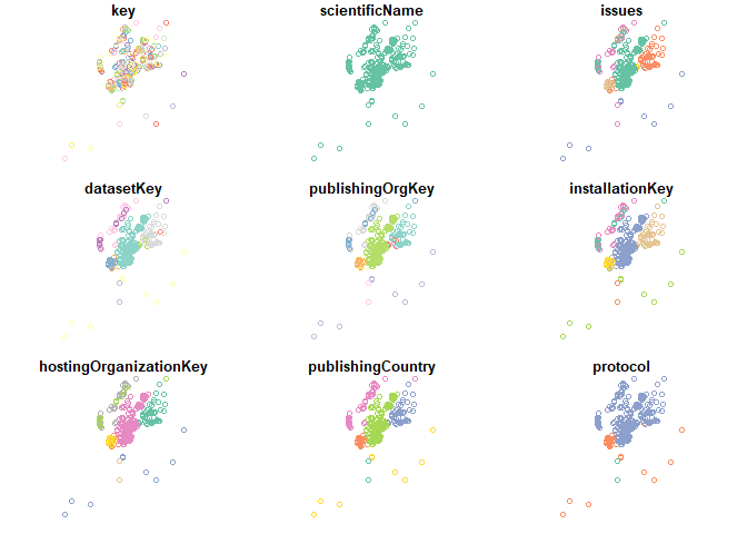
Note that we use st_geometry() here rather than just
plot(howler_sf). The latter would attempt to produce a
separate map for every column in the data frame — which is technically
valid R but not what we want right now.
Even this basic map is informative. Records cluster in certain areas, and large parts of the species’ potential range look empty. This could reflect genuine habitat preferences. For example, howlers are forest-dependent and associate strongly with lowland and mid-elevation tropical forest (Fedigan & Jack 2001). But it could equally reflect where researchers happened to work, or where road access made surveys feasible.
This ambiguity (signal versus sampling) is one of the central challenges of biodiversity informatics, and we’ll address it directly in Module 5.
Exploring the data
Let’s look at a few useful fields to get a feel for what we’re working with.
# Which countries do records come from?
table(howler_sf$countryCode)
##
## CR EC HN MX NI PA
## 239 5 3 4 12 37# Date range of records
range(howler_sf$eventDate, na.rm = TRUE)## [1] "2026-01-01T08:34:35" "2026-02-23T06:09:37"# How many records lack a date?
sum(is.na(howler_sf$eventDate))## [1] 0Records span multiple decades and countries, a reminder that GBIF aggregates historical museum specimens alongside recent field surveys. A specimen collected in 1952 and a camera trap photo from last year sit in the same dataset, treated equivalently unless you filter by date or some other criteria. For modelling present-day distributions, this is worth keeping in mind.
A note on data quality
It’s tempting to treat downloaded data as ready to use. It isn’t, at least not yet. GBIF records have been shown to contain substantial proportions of coordinate errors, including points placed in the ocean, at country centroids (a common georeferencing shortcut), and at 0°, 0° in the Gulf of Guinea (Maldonado et al. 2015). These are not rare edge cases; they’re common enough to meaningfully bias analyses if left unchecked.
For now, we’re just getting familiar with how spatial data looks and behaves in R. Cleaning and quality control come in Module 7.
References
Chamberlain, S. & Boettiger, C. (2017). R Python, and Ruby clients for the GBIF species occurrence API. PeerJ Preprints, 5, e3304v1.
Fedigan, L.M. & Jack, K. (2001). Neotropical primates in a regenerating Costa Rican dry forest: a comparison of howler and capuchin population patterns. International Journal of Primatology, 22, 689–713.
Maldonado, C., Molina, C.I., Zizka, A., Persson, C., Taylor, C.M., Albán, J., Chilquillo, E., Rønsted, N. & Antonelli, A. (2015). Estimating species diversity and distribution in the era of Big Data. Global Ecology and Biogeography, 24, 1305–1317.
Pebesma, E. (2018). Simple features for R: standardized support for spatial vector data. The R Journal, 10, 439–446.