Coordinates and projections

For this module, you’ll need the following packages:

sf
rgbif
rnaturalearth
rnaturalearthdata

At some point, you will plot spatial data and notice that something looks wrong. Layers don’t line up, points appear in the ocean, or your map looks oddly stretched. Nine times out of ten, the culprit is coordinate systems. This module explains what they are, why they matter, and how to fix the problems they cause.

The fundamental problem: Earth is not flat

This sounds obvious, but it has real consequences. The Earth is roughly spherical (technically an oblate spheroid), slightly squashed at the poles. Your screen is resolutely flat. Representing a curved surface in two dimensions always requires compromise, and that compromise is formalised through two related concepts:

Coordinate Reference Systems (CRS) define how locations on Earth are described. They are mathematical models of Earth’s shape and the framework for specifying positions on it.

Projections define how those 3D coordinates are flattened onto a 2D map. Every projection preserves some properties (shape, area, distance, direction) and distorts others. The Mercator projection — the one that makes Greenland look roughly the same size as Africa — preserves shape locally but massively distorts area at high latitudes. Equal-area projections do the opposite. There is no perfect projection, only appropriate ones for different purposes (Snyder 1987).

In ecology, this matters most when you’re measuring distances or areas, combining datasets from different sources, or doing anything where spatial accuracy affects the result. A distance calculated in degrees of latitude/longitude is not the same as one calculated in metres, and treating them as equivalent is a common source of silent error.

Latitude, longitude, and WGS84

Most GBIF data and most GPS receivers use latitude and longitude in the WGS84 coordinate system. WGS84 (World Geodetic System 1984) is the global standard used in satellite navigation and geodesy. In R, you’ll often see it referred to by its EPSG code: 4326. EPSG codes are standardised numeric identifiers for coordinate reference systems; a full searchable list is at epsg.io.

Let’s check the CRS of our howler monkey data from Module 2:

st_crs(howler_sf)

## Coordinate Reference System:
##   User input: EPSG:4326 
##   wkt:
## GEOGCRS["WGS 84",
##     ENSEMBLE["World Geodetic System 1984 ensemble",
##         MEMBER["World Geodetic System 1984 (Transit)"],
##         MEMBER["World Geodetic System 1984 (G730)"],
##         MEMBER["World Geodetic System 1984 (G873)"],
##         MEMBER["World Geodetic System 1984 (G1150)"],
##         MEMBER["World Geodetic System 1984 (G1674)"],
##         MEMBER["World Geodetic System 1984 (G1762)"],
##         MEMBER["World Geodetic System 1984 (G2139)"],
##         MEMBER["World Geodetic System 1984 (G2296)"],
##         ELLIPSOID["WGS 84",6378137,298.257223563,
##             LENGTHUNIT["metre",1]],
##         ENSEMBLEACCURACY[2.0]],
##     PRIMEM["Greenwich",0,
##         ANGLEUNIT["degree",0.0174532925199433]],
##     CS[ellipsoidal,2],
##         AXIS["geodetic latitude (Lat)",north,
##             ORDER[1],
##             ANGLEUNIT["degree",0.0174532925199433]],
##         AXIS["geodetic longitude (Lon)",east,
##             ORDER[2],
##             ANGLEUNIT["degree",0.0174532925199433]],
##     USAGE[
##         SCOPE["Horizontal component of 3D system."],
##         AREA["World."],
##         BBOX[-90,-180,90,180]],
##     ID["EPSG",4326]]

You should see WGS84 in the output. If a dataset has no CRS listed or returns NA that’s a warning sign. You’ll need to establish what system the coordinates are actually in before doing anything spatial.

Why mismatched CRS causes problems

When you combine two datasets with different coordinate systems, R does not automatically know they should line up. It treats the coordinate numbers as directly comparable even when they refer to completely different spatial frameworks. The result can look absurd.

Let’s demonstrate. We’ll take our howler monkey data (WGS84, in decimal degrees) and a Costa Rica polygon that we’ve deliberately reprojected into a projected coordinate system using metres, the Costa Rica Topo Map projection (EPSG:5367). Because one dataset uses degrees and the other uses metres, the numbers are completely different in scale and meaning.

library(rnaturalearth)
library(rnaturalearthdata)

world <- ne_countries(scale = "medium", 
                      returnclass = "sf")
cr    <- world[world$name == "Costa Rica", ]

# Reproject Costa Rica into a metre-based projected system
cr_proj <- st_transform(cr, 5367)

# Now try to plot both layers together
plot(st_geometry(cr_proj), 
     main = "A CRS mismatch in action")
plot(st_geometry(howler_sf), 
     add = TRUE, col = "red", 
     pch = 19, 
     cex = 0.5)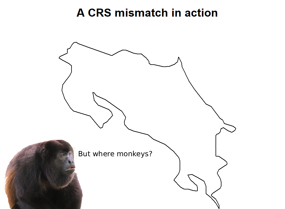

# Compare coordinate ranges
st_bbox(howler_sf)

##       xmin       ymin       xmax       ymax 
## -94.506286  -3.743768 -77.368218  18.371243

st_bbox(cr_proj)

##      xmin      ymin      xmax      ymax 
##  291391.7  892546.0  657688.2 1237763.0

hist(st_coordinates(howler_sf)[,1],
     main = "Howler longitude (degrees)",
     xlab = "Longitude")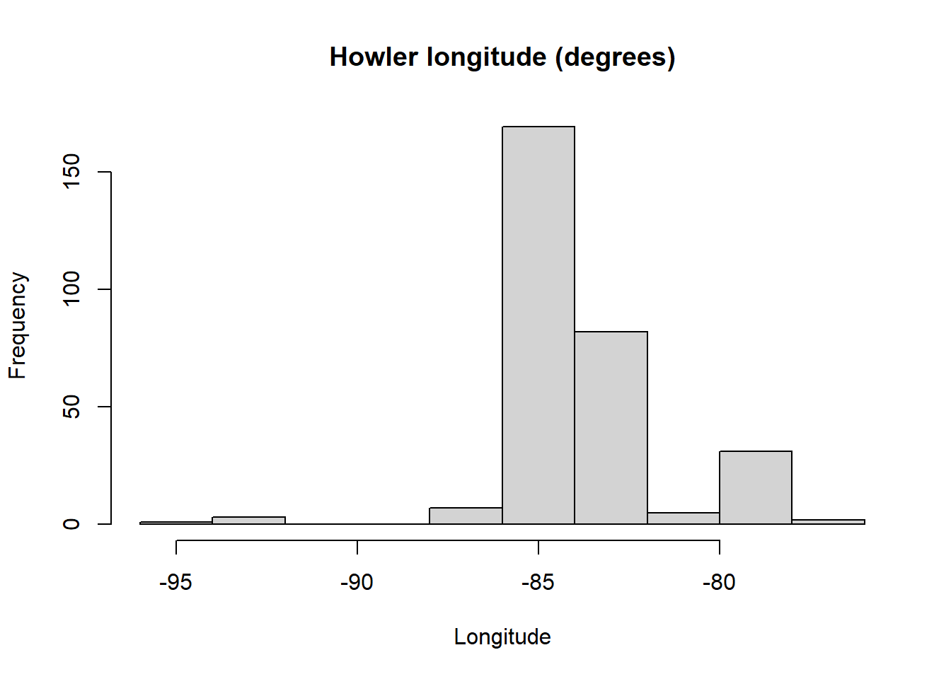

hist(st_coordinates(cr_proj)[,1],
     main = "Costa Rica CRS (metres)",
     xlab = "Projected X coordinate")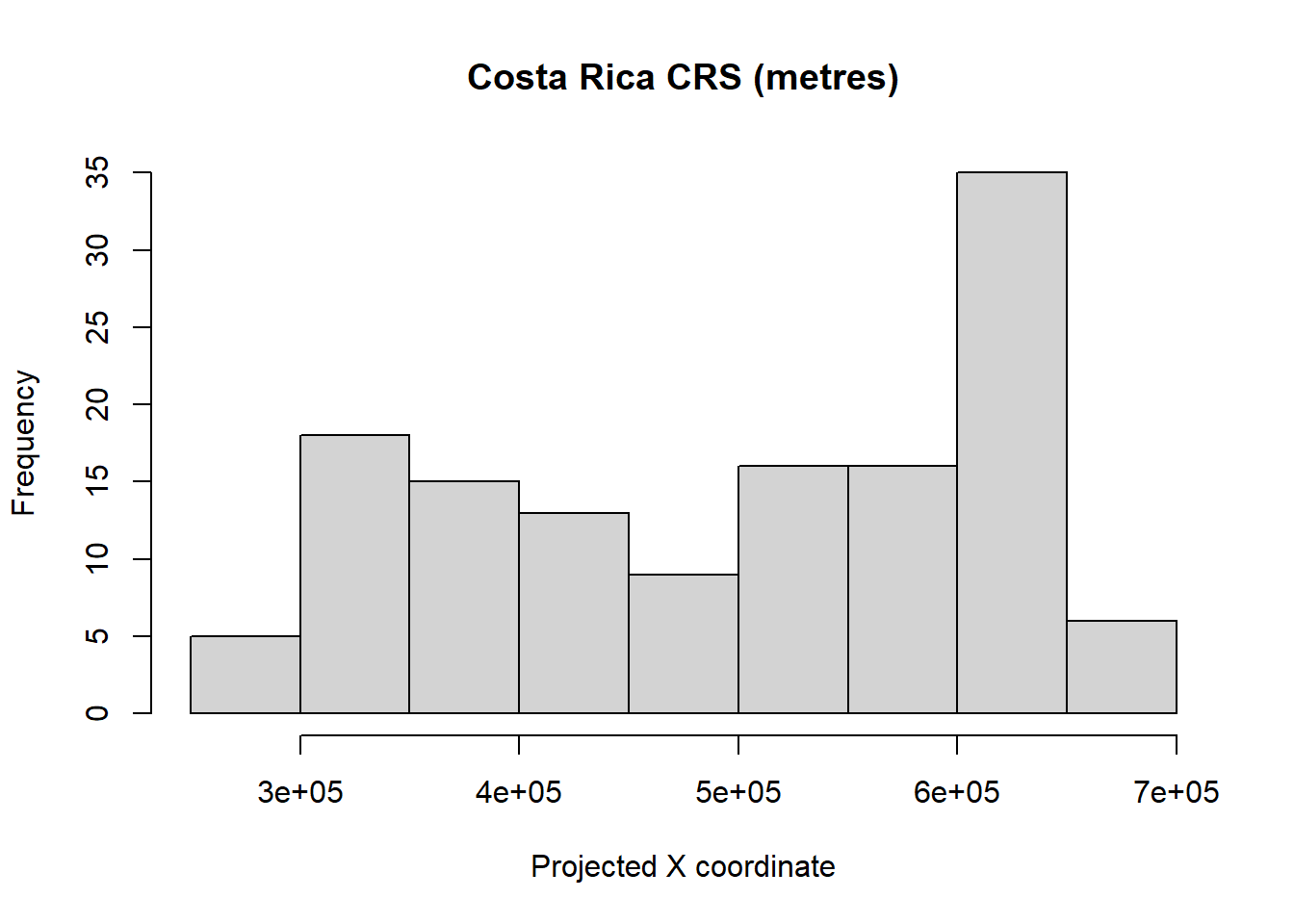

The howler points appear nowhere near Costa Rica. This is not a data error - it is a coordinate system mismatch. The polygon coordinates are in metres (EPSG:5367); the point coordinates are in degrees (EPSG:4326). R plots both on the same axis without complaint, because it doesn’t know they’re incompatible.

Whenever layers fail to align, this is the first thing to check:

st_crs(cr_proj)$epsg

## [1] 5367

st_crs(howler_sf)$epsg

## [1] 4326

Fixing it: reprojection

The solution is st_transform(). You pick a target CRS and reproject one layer to match. Since we’ll mostly work in WGS84 (it’s what GBIF uses, and it’s what most global environmental datasets use) the simplest fix is to transform the polygon back:

cr_wgs84 <- st_transform(cr_proj, 4326)

plot(st_geometry(cr_wgs84), 
     main = "After reprojection — layers now align")
plot(st_geometry(howler_sf), 
     add = TRUE, 
     col = "red", 
     pch = 19, cex = 0.6)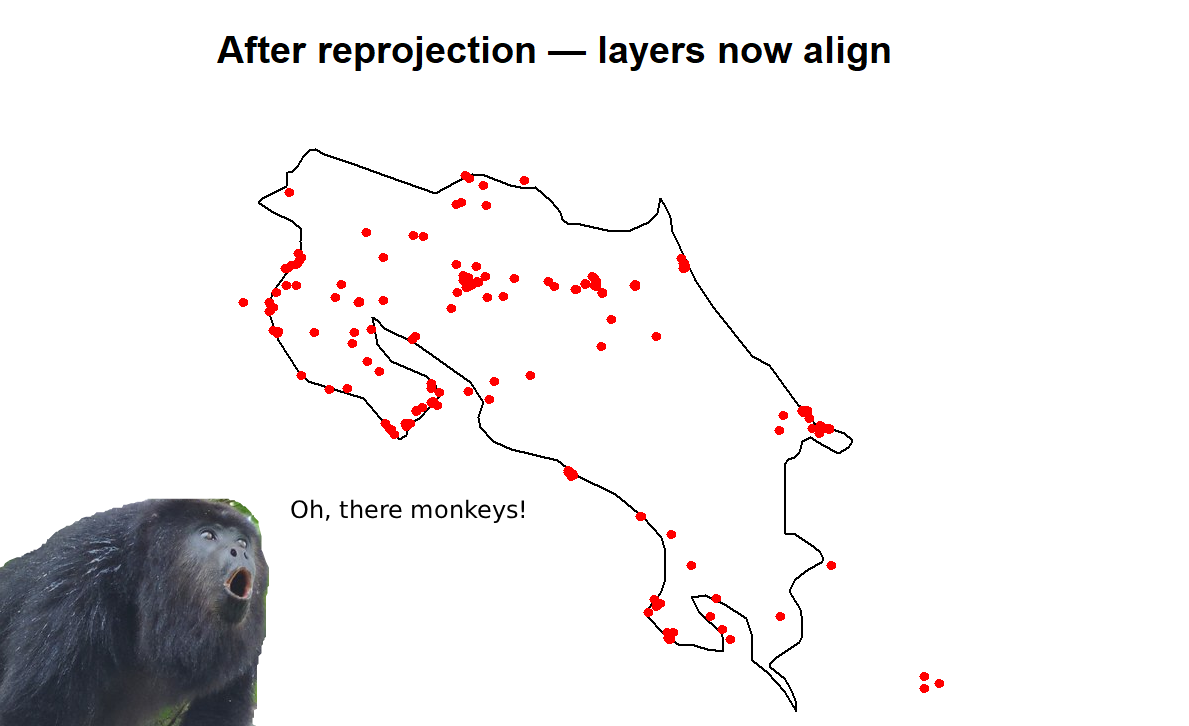

The layers now align. You can also see that some howler records fall outside Costa Rica because we downloaded the full global dataset in Module 2, not just Costa Rica records. We’ll fix that in Module 4.

Which projection should I use?

For large-scale analyses (continental or global), WGS84 (EPSG:4326) is usually appropriate and keeps everything consistent with source data. For regional analyses where accurate distances or areas are needed, such as spatial thinning, home range estimation, or connectivity modelling, a projected system in metres is more appropriate.

For Central America and Costa Rica specifically, sensible options include EPSG:5367 (Costa Rica Topo Map, national standard), or EPSG:32616 (UTM Zone 16N, metres, widely used in ecological research in the region).

The key rule is simple: all layers in an analysis must use the same CRS. Check every time you read in new data, and transform early rather than late. Future you will be grateful.

References

Snyder, J.P. (1987). Map Projections: A Working Manual. US Geological Survey Professional Paper 1395. US Government Printing Office, Washington DC.

← Previous Next →