Points, polygons, and rasters
For this module, you’ll need the following packages:
sfrgbifrnaturalearthrnaturalearthdataterrageodata
So far we’ve worked with occurrence points and learned how coordinate systems work. But a single layer of data rarely tells the whole ecological story. To understand why species are where they are, we need to combine multiple layers: the species records, a boundary defining our study area, and environmental data describing the landscape. This module brings all three together.
Three layers, one framework
Almost every spatial ecology workflow combines the same fundamental data types:
- Points; individual observations at specific locations (species records, survey sites, GPS tracks)
- Polygons; bounded areas representing regions, habitats, or administrative units
- Rasters; continuous environmental surfaces (elevation, temperature, land cover, vegetation index)
Together, these form the backbone of landscape ecology, species distribution modelling, and conservation planning. The field of macroecology, or understanding broad-scale patterns in biodiversity, is built almost entirely on combining these data types at regional to global scales (Gaston & Blackburn 2000). Getting comfortable with how they interact is one of the most transferable skills in ecological data analysis.
Step 1: Define the study region
We’ll continue to focus on Costa Rica for the rest of this course. Straddling Central America between roughly 8–11°N, Costa Rica packs an extraordinary range of habitats into a small area, including Pacific dry forest, Caribbean rainforest, highland cloud forest, mangroves, and everything in between. It is one of the most biodiverse countries on Earth per unit area, and the mantled howler monkey (Alouatta palliata) is one of its most visible and well-studied forest mammals. Costa Rica has good biodiversity data infrastructure, partly as a legacy of long-running primate research programmes (Fedigan & Jack 2001).
library(sf)
library(rnaturalearth)
library(rnaturalearthdata)

world  <- ne_countries(scale = "medium", returnclass = "sf")
region <- world[world$name == "Costa Rica", ]

plot(st_geometry(region), main = "Costa Rica")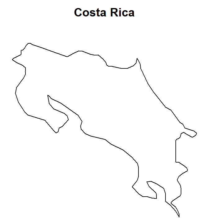
Step 2: Download howler monkey records for Costa Rica
Now we’ll download occurrence records filtered to Costa Rica at
source. Specifying country = "CR" is more efficient than
downloading the full global dataset and clipping it afterwards —
especially as the species occurs across much of Central America.
library(rgbif)

species <- occ_search(
  scientificName = "Alouatta palliata",
  country = "CR",
  limit = 2000,
  hasCoordinate = TRUE
)

howler_sf <- st_as_sf(
  species$data,
  coords = c("decimalLongitude", "decimalLatitude"),
  crs = 4326
)

nrow(howler_sf)
## [1] 2000plot(st_geometry(region), main = "Mantled howler monkey — Costa Rica")
plot(st_geometry(howler_sf), add = TRUE, col = "red", pch = 16, cex = 0.5)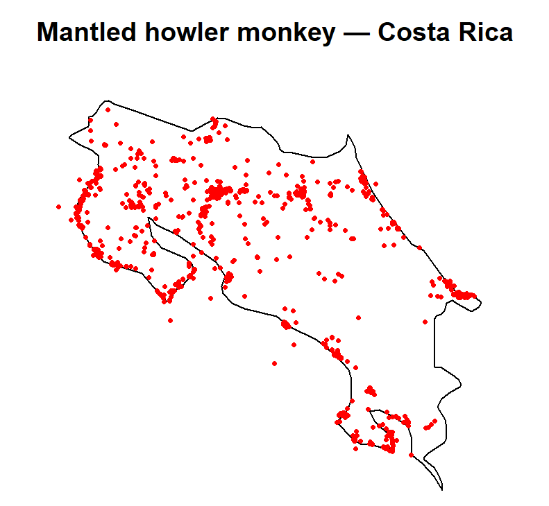
Records are not evenly spread. You’ll likely see clusters near the Osa Peninsula, around research stations in Guanacaste, and along the Caribbean lowlands. These are areas with long histories of primate research. Gaps elsewhere may reflect genuine habitat limits, but also simply where researchers have and haven’t worked. We’ll investigate this properly in Module 5.
Step 3: Download elevation data
Environmental rasters give us the “why” behind species distributions. We’ll start with elevation — one of the most powerful predictors of species occurrence in tropical systems, because it correlates tightly with temperature, rainfall, and vegetation structure (Rahbek et al. 2019). A species recorded predominantly at low elevations might be limited by cold temperatures at altitude, or by the distribution of the forest types it depends on.
library(geodata)
library(terra)

geodata_path(".")   # sets where downloaded files are cached

elev <- elevation_global(res = 10)   # 10-minute resolution global elevation model
plot(elev, main = "Global elevation")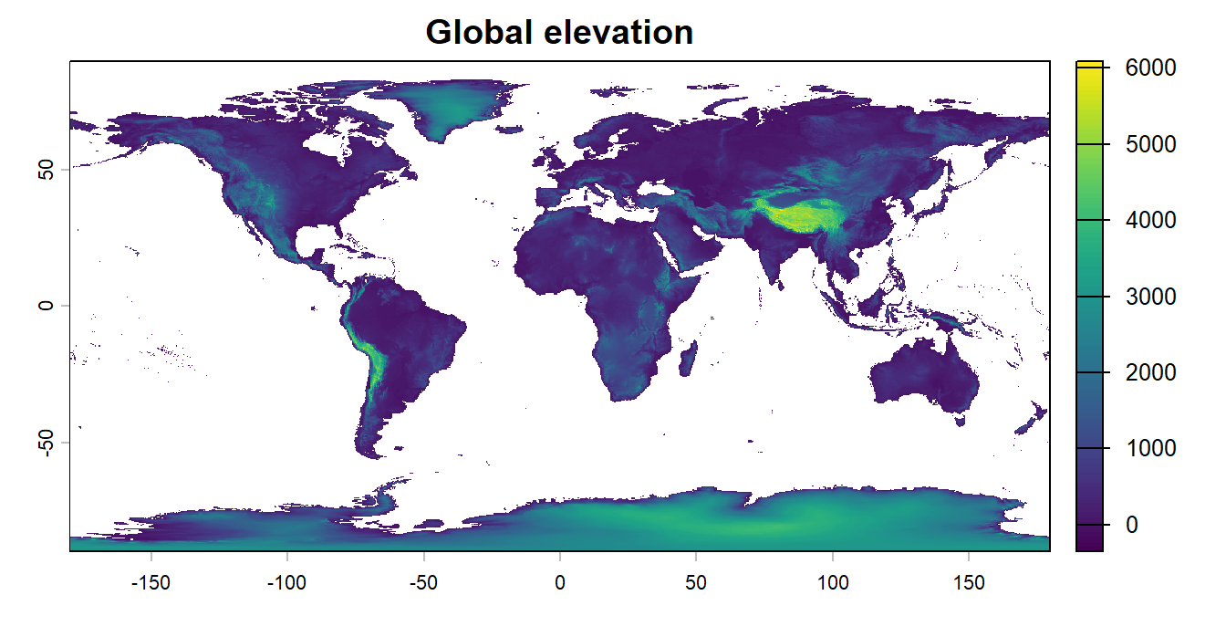
That’s the entire world, which is considerably more than we need. Time to cut it down.
Step 4: Crop and mask to the study region
Two operations are useful here, almost always applied in sequence:
crop()trims the raster to the bounding box of the polygon. This is quick, but includes cells that fall outside the polygon boundary.mask()sets any cells outside the polygon to NA, removing data beyond the border.
Always check coordinate systems match before combining spatial layers:
crs(elev, describe = TRUE)## name authority code area extent
## 1 WGS 84 EPSG 4326 World -180, 180, -90, 90st_crs(region)$input## [1] "WGS 84"Both should be WGS84. If not, transform before proceeding.
elev_cr <- crop(elev, vect(region))
elev_cr <- mask(elev_cr, vect(region))

plot(elev_cr, main = "Elevation — Costa Rica (m)")
Costa Rica’s topography is immediately apparent: a central cordillera running roughly northeast to southwest, with lower-lying areas to the Pacific coast and the Caribbean lowlands. Howler monkeys are primarily lowland and mid-elevation animals, typically recorded below about 1,500 m, where lowland and premontane wet forests dominate (Estrada et al. 2006).
Step 5: Bring it all together
Now we can overlay all three layers to see our species distribution in its environmental context.
plot(elev_cr, main = "Mantled howler monkey — elevation context")
plot(st_geometry(region), add = TRUE, border = "black", lwd = 1.5)
plot(st_geometry(howler_sf), add = TRUE, col = "red", pch = 16, cex = 0.5)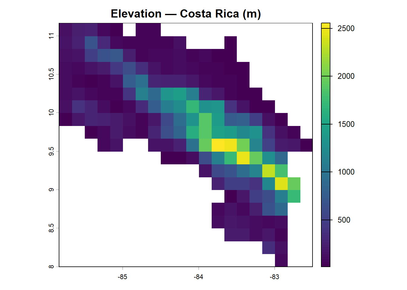
This is the basic template for spatial ecology: an environmental layer providing landscape context, a boundary defining the study region, and species observations embedded within it. Everything we do for the rest of this course builds on exactly this structure.
What does this tell us?
Even from this map, you can start forming hypotheses. Are howler records more common in the lowlands? Do they avoid the central mountains? Are there coastal clusters that might reflect accessible survey sites rather than real density?
Don’t try to answer those questions from the map alone — that’s what the analysis is for. But this is the process: map the data, form hypotheses, then test them rigorously. Spatial ecology at its best is just the scientific method with an explicit geography.
References
Estrada, A., Garber, P.A., Pavelka, M. & Luecke, L. (eds.) (2006). New Perspectives in the Study of Mesoamerican Primates. Springer, New York.
Fedigan, L.M. & Jack, K. (2001). Neotropical primates in a regenerating Costa Rican dry forest: a comparison of howler and capuchin population patterns. International Journal of Primatology, 22, 689–713.
Gaston, K.J. & Blackburn, T.M. (2000). Pattern and Process in Macroecology. Blackwell Science, Oxford.
Rahbek, C., Borregaard, M.K., Colwell, R.K., Dalsgaard, B., Holt, B.G., Morueta-Holme, N., Nogues-Bravo, D., Whittaker, R.J. & Fjeldså, J. (2019). Humboldt’s enigma: what causes global patterns of mountain biodiversity? Science, 365, 1108–1113.