Working with environmental data
For this module, you’ll need the following packages:
sfterrageodatarnaturalearthrnaturalearthdata
In Module 5 we asked whether the patterns in our howler monkey data reflect real ecology or sampling effort. To start answering that — and to eventually build a species distribution model — we need environmental data describing what conditions actually exist across the landscape.
This module covers downloading, inspecting, and preparing the environmental layers we’ll use throughout the rest of the course. By the end, you’ll have a multi-layer raster stack covering Costa Rica that’s ready for analysis.
Why environmental data?
The dominant theory in species distribution modelling is Hutchinson’s n-dimensional hypervolume — the idea that a species can persist anywhere that its full set of environmental requirements are met (Hutchinson 1957). In practice this is simplified considerably, but the core logic holds: species are found where their environment suits them. To predict where a species might occur, we need to know both where it has been recorded and what the environment looks like everywhere else.
The two most commonly used environmental data sources in SDM work are elevation and climate — particularly the WorldClim bioclimatic variables, which we’ll use here.
Loading packages and defining the study region
library(sf)
library(terra)
library(geodata)
library(rnaturalearth)
library(rnaturalearthdata)
world <- ne_countries(scale = "medium", returnclass = "sf")
region <- world[world$name == "Costa Rica", ]
region_vect <- vect(region) # terra needs SpatVector, not sf
region_bbox <- st_bbox(region) # bounding box for croppingElevation
We already met elevation in Module 4. Let’s download it properly and prepare it for use alongside climate data.
geodata_path(".")

elev    <- elevation_global(res = 10)
elev_cr <- crop(elev, region_vect)
elev_cr <- mask(elev_cr, region_vect)

plot(elev_cr, main = "Elevation — Costa Rica (m)")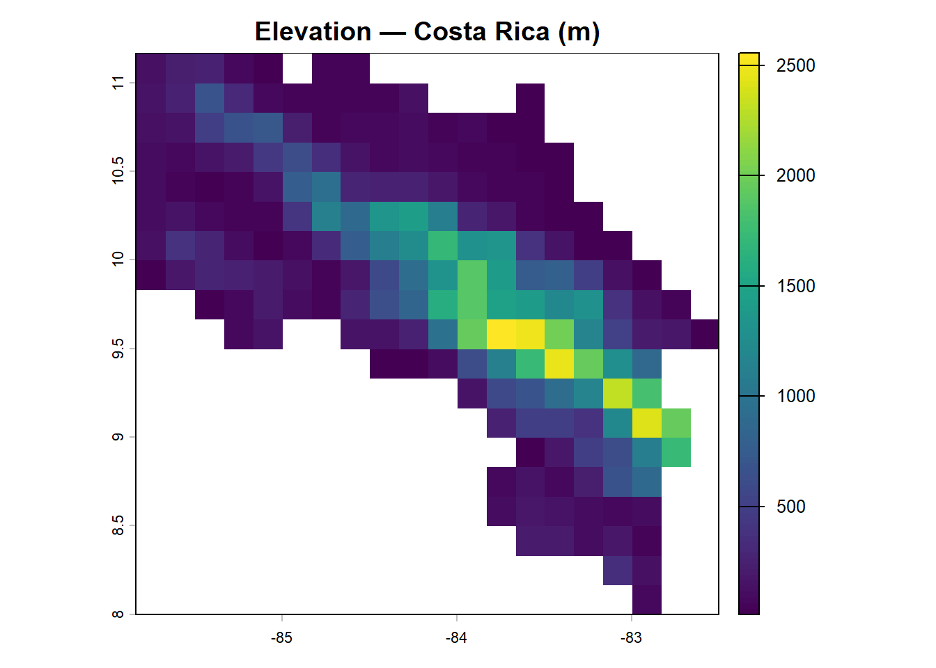
# Quick summary of elevation values
summary(values(elev_cr), na.rm = TRUE)
## wc2.1_10m_elev
## Min. : 11.0
## 1st Qu.: 75.5
## Median : 176.0
## Mean : 485.1
## 3rd Qu.: 699.0
## Max. :2555.0
## NA's :185Costa Rica ranges from sea level to over 3,800 m at Cerro Chirripó. That’s a remarkable range for a country roughly the size of West Virginia, and it’s a large part of why Costa Rica is so biodiverse — it compresses multiple elevational zones and climate regimes into a small area (Janzen 1983).
WorldClim bioclimatic variables
WorldClim provides 19 bioclimatic variables derived from monthly temperature and precipitation data, interpolated from global weather station networks (Fick & Hijmans 2017). They were designed specifically for species distribution modelling and are now one of the most widely used environmental datasets in ecology. The 19 variables cover things like:
- bio01: Mean annual temperature
- bio04: Temperature seasonality (standard deviation × 100)
- bio12: Annual precipitation
- bio15: Precipitation seasonality (coefficient of variation)
- bio17: Precipitation of the driest quarter
A full description of all 19 variables is at worldclim.org/data/bioclim.html.
Note that temperature variables are stored in °C × 10 — so a value of 245 means 24.5°C. This is a legacy convention from when integer storage saved meaningful disk space. Divide by 10 to get degrees Celsius.
# Set download = TRUE the first time, then FALSE to use cached files
clim <- worldclim_global(var = 'bio', res = 10, download = FALSE, path = 'data')

# Rename to cleaner labels
names(clim) <- c(paste0('bio0', 1:9), paste0('bio', 10:19))

# Crop and mask to Costa Rica
clim_cr <- crop(clim, region_vect)
clim_cr <- mask(clim_cr, region_vect)

clim_cr
## class : SpatRaster
## size : 19, 20, 19 (nrow, ncol, nlyr)
## resolution : 0.1666667, 0.1666667 (x, y)
## extent : -85.83333, -82.5, 8, 11.16667 (xmin, xmax, ymin, ymax)
## coord. ref. : lon/lat WGS 84 (EPSG:4326)
## source(s) : memory
## names : bio01, bio02, bio03, bio04, bio05, bio06, ...
## min values : 11.86418, 6.975149, 71.24990, 52.38264, 17.60925, 5.98050, ...
## max values : 27.48187, 11.785084, 82.39379, 94.06358, 35.58375, 21.73693, ...Let’s plot a few variables to get a feel for the data.
# Mean annual temperature (divide by 10 for °C)
plot(clim_cr[['bio01']] / 10,
     main = "Mean annual temperature (°C)")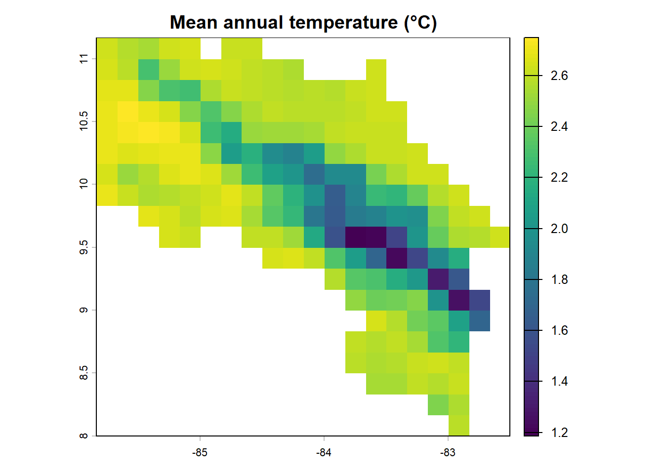
# Annual precipitation (mm)
plot(clim_cr[['bio12']],
     main = "Annual precipitation (mm)")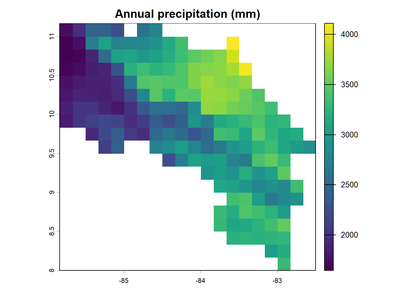
# Precipitation seasonality
plot(clim_cr[['bio15']],
     main = "Precipitation seasonality")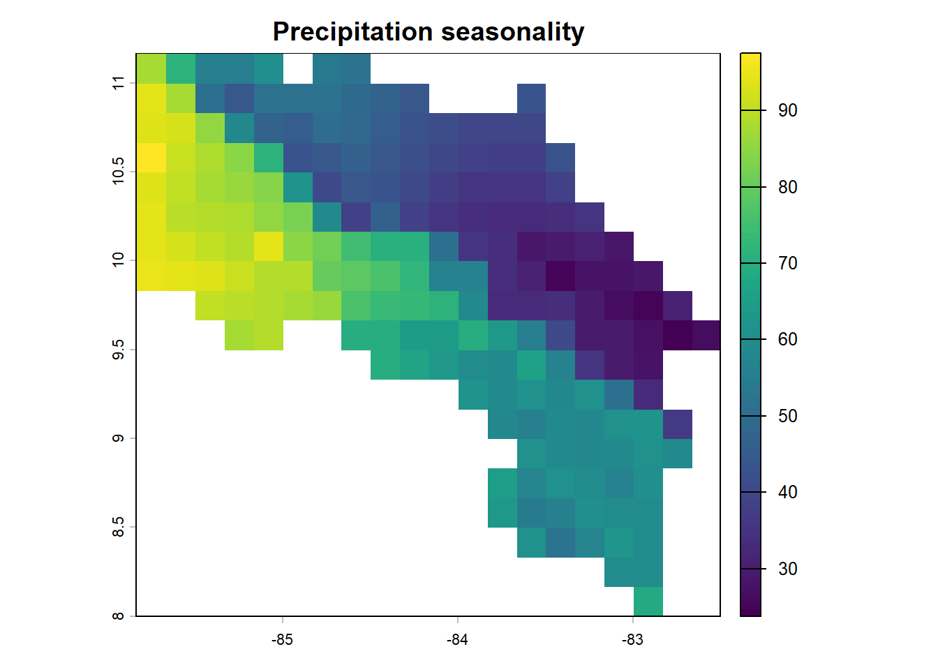
Notice how different variables tell different stories about the landscape. Temperature broadly tracks elevation — cooler highlands, warmer coasts. Precipitation is patchier, reflecting the complex rain shadow effects of the central mountains, which create a drier Pacific slope and a wetter Caribbean side.
Checking that layers align
Before stacking and combining layers, we need to confirm that they share the same resolution, extent, and CRS. Layers that don’t align can’t be combined without error.
# Resolution
res(elev_cr)
## [1] 0.1666667 0.1666667res(clim_cr)## [1] 0.1666667 0.1666667# CRS
crs(elev_cr, describe = TRUE)## name authority code area extent
## 1 WGS 84 EPSG 4326 World -180, 180, -90, 90crs(clim_cr, describe = TRUE)## name authority code area extent
## 1 WGS 84 EPSG 4326 World -180, 180, -90, 90The resolutions should both be approximately 0.167° (10 arc-minutes). If they differ, we need to resample. Here we resample elevation to exactly match the climate grid, which ensures perfect alignment.
elev_resamp <- terra::resample(elev_cr, clim_cr, method = 'bilinear')

# Confirm match
res(elev_resamp)
## [1] 0.1666667 0.1666667res(clim_cr)## [1] 0.1666667 0.1666667Now we can stack them.
env_stack <- c(clim_cr, elev_resamp)
names(env_stack)[20] <- 'elev'

nlyr(env_stack)   # should be 20
## [1] 20names(env_stack)## [1] "bio01" "bio02" "bio03" "bio04" "bio05" "bio06" "bio07" "bio08" "bio09"
## [10] "bio10" "bio11" "bio12" "bio13" "bio14" "bio15" "bio16" "bio17" "bio18"
## [19] "bio19" "elev"Extracting values at points
To check everything’s working, let’s extract environmental values at a few howler monkey locations.
library(rgbif)## Warning: package 'rgbif' was built under R version 4.5.3species <- occ_search(
scientificName = "Alouatta palliata",
country = "CR",
limit = 2000,
hasCoordinate = TRUE
)
howler_sf <- st_as_sf(
species$data,
coords = c("decimalLongitude", "decimalLatitude"),
crs = 4326
)## ID bio01 bio02 bio03 bio04 bio05 bio06 bio07 bio08
## 1 1 27.36959 10.549562 75.11258 81.58629 35.13100 21.08600 14.04500 26.83204
## 2 2 27.23806 10.420375 75.84937 76.99428 34.80850 21.07025 13.73825 26.75783
## 3 3 26.26099 7.571301 75.19080 79.95874 31.53285 21.46340 10.06945 26.43492
## 4 4 25.65477 8.225204 78.03919 73.83220 31.10515 20.56531 10.53984 24.88519
## 5 5 25.44864 8.554354 76.85506 77.53883 31.35675 20.22625 11.13050 25.61754
## bio09 bio10 bio11 bio12 bio13 bio14 bio15 bio16 bio17 bio18 bio19
## 1 27.65667 28.55733 26.52408 1879 366 4 87.82879 944 18 292 487
## 2 27.52625 28.33908 26.41275 1871 356 6 85.86667 922 25 298 486
## 3 26.94654 27.37181 25.36921 3768 510 123 37.64306 1247 479 582 1175
## 4 26.21247 26.62674 24.76807 2977 316 144 23.76402 896 505 603 819
## 5 26.12367 26.52971 24.59117 3621 457 115 37.58236 1227 414 566 991
## elev
## 1 25
## 2 40
## 3 19
## 4 174
## 5 176Each row is an occurrence point; each column is an environmental variable at that location. This is the foundation of species distribution modelling — the numerical pairing of “where was the species?” with “what was the environment there?”
Save your work
We’ll use these objects in every subsequent module.
terra::writeRaster(env_stack, 'data/env_stack.tif', overwrite = TRUE)
terra::writeRaster(clim_cr,   'data/clim_cr.tif',   overwrite = TRUE)
# Note: region_vect is a terra SpatVector and cannot be saved with save() —
# terra's external pointer objects become invalid when serialised.
# We save region (an sf object) and recreate region_vect with vect() as needed.
save(region, region_bbox, file = 'data/region.RData')
Exercise
- Plot
bio04(temperature seasonality). Where in Costa Rica is temperature most seasonal? Does this make geographical sense given what you know about the country’s climate? - Use
terra::extract()to get the mean annual temperature (bio01 / 10) at all howler locations. What is the range of temperatures where howlers have been recorded? Does this align with what you’d expect for a tropical forest species? - Use
terra::global(clim_cr[['bio12']], fun = 'mean', na.rm = TRUE)to calculate mean annual precipitation across Costa Rica. Then do the same forbio15(precipitation seasonality). Which part of the country do you think is the most challenging environment for a forest-dependent species?
References
Fick, S.E. & Hijmans, R.J. (2017). WorldClim 2: new 1-km spatial resolution climate surfaces for global land areas. International Journal of Climatology, 37, 4302–4315.
Hutchinson, G.E. (1957). Concluding remarks. Cold Spring Harbor Symposia on Quantitative Biology, 22, 415–427.
Janzen, D.H. (1983). No park is an island: increase in interference from outside as park size decreases. Oikos, 41, 402–410.