Preparing occurrence data for modelling
For this module, you’ll need the following packages:
sfterradplyrrgbifrnaturalearthrnaturalearthdata
In Module 5 we established that GBIF data is a mix of ecological signal and observation effort. In Module 6 we assembled our environmental layers. Now we need to bridge the two: prepare the occurrence data so that it’s clean, spatially appropriate, and paired with environmental values — ready to feed into a statistical model.
This step is often glossed over in tutorials. That’s a mistake. As the saying goes in data science: garbage in, garbage out. An SDM built on uncleaned data can perform well statistically while being ecologically meaningless (Hijmans & Elith 2019).
Load the data
library(sf)
library(terra)
library(dplyr)
load('data/region.RData')
env_stack <- terra::rast('data/env_stack.tif')And re-download the howler monkey records if they’re not already in your environment:
library(rgbif)

species <- occ_search(
  scientificName = "Alouatta palliata",
  country = "CR",
  limit = 2000,
  hasCoordinate = TRUE
)

howler_sf <- st_as_sf(
  species$data,
  coords = c("decimalLongitude", "decimalLatitude"),
  crs = 4326
)nrow(howler_sf)## [1] 2000Step 1: Remove duplicate records
GBIF aggregates records from many sources, and the same observation can appear multiple times — submitted by different institutions, transcribed from the same museum specimen, or simply repeated. Duplicates inflate the apparent importance of heavily recorded locations.
We’ll round coordinates to three decimal places (roughly 100 m resolution) and remove any records that share identical rounded positions.
howler_sf <- howler_sf %>%
  mutate(
    lon_round = round(st_coordinates(.)[, 1], 3),
    lat_round = round(st_coordinates(.)[, 2], 3)
  ) %>%
  distinct(lon_round, lat_round, .keep_all = TRUE)

nrow(howler_sf)
## [1] 1399Step 2: Remove records with imprecise coordinates
Some GBIF records have whole-number coordinates — e.g. exactly 9.0°N, 84.0°W. These often represent rough centroids or poorly georeferenced historical specimens rather than real GPS locations. We’ll flag and remove them.
coords <- as.data.frame(st_coordinates(howler_sf))
names(coords) <- c("lon", "lat")

# Flag records where both coordinates are whole numbers
imprecise <- coords$lon == round(coords$lon) & coords$lat == round(coords$lat)
cat(sum(imprecise), "records with whole-number coordinates removed\n")
## 0 records with whole-number coordinates removedhowler_sf <- howler_sf[!imprecise, ]
# Also remove any records at exactly 0, 0 — a classic georeferencing error
zero_coords <- coords$lon == 0 & coords$lat == 0
howler_sf <- howler_sf[!zero_coords, ]
nrow(howler_sf)## [1] 1399Step 3: Clip to the study region
Although we filtered by country = "CR" when downloading,
GBIF coordinates are not always precise enough to guarantee every point
actually falls inside the country polygon. Some records sit just
offshore, straddle a border, or have coordinates that place them in a
neighbouring country due to georeferencing error. Before doing anything
spatial, we should remove these.
# Keep only points that fall within the Costa Rica polygon
howler_sf <- howler_sf[st_within(howler_sf, region, sparse = FALSE)[, 1], ]

nrow(howler_sf)
## [1] 1125st_within() returns TRUE only for points that fall
strictly inside the polygon. Any points on the coast, in the ocean, or
across the border are silently removed. Always do this before thinning —
there’s no point thinning data you’d discard anyway.
Step 4: Spatial thinning
Even after removing duplicates, GBIF data is spatially uneven. Decades of research near La Selva Biological Station and Corcovado National Park mean those areas are far more densely sampled than remote highland zones. If we feed this directly into a model, the model will effectively learn “this species is associated with areas that ecologists like to visit” — not what we’re after.
Spatial thinning addresses this by keeping at most one record per raster grid cell. It’s worth being clear about why this is appropriate here, and when it might not be.
The rasters we’re using are at 10-minute resolution — each cell covers roughly 18 × 18 km at the equator. Two occurrence points falling in the same cell will always receive identical environmental predictor values when we extract from those rasters, because they occupy the same pixel. Keeping both adds nothing to the model: it’s the same information twice, just inflating the sample size and the apparent weight of heavily sampled locations. One record per cell is therefore not discarding ecological information — it’s discarding redundancy.
If you were working with higher-resolution rasters (1 km WorldClim, LiDAR-derived canopy height, etc.), finer-scale thinning would be appropriate. If you were using very coarse rasters (0.5° or lower), thinning to one point per cell would be extremely aggressive and genuinely wasteful. The right thinning resolution is the raster resolution.
ref_grid <- env_stack[[1]]

# Find which raster cell each presence point falls in
howler_vect    <- vect(howler_sf)
cells          <- terra::cellFromXY(ref_grid, geom(howler_vect)[, c('x', 'y')])
howler_sf$cell <- cells

# Keep one record per cell
howler_thinned <- howler_sf %>%
  group_by(cell) %>%
  slice(1) %>%
  ungroup() %>%
  select(-cell)

nrow(howler_thinned)
## [1] 121# Visualise before and after
par(mfrow = c(1, 2))
plot(st_geometry(region), main = paste("Before thinning\n(n =", nrow(howler_sf), ")"))
plot(st_geometry(howler_sf), add = TRUE, col = "tomato", pch = 19, cex = 0.4)
plot(st_geometry(region), main = paste("After thinning\n(n =", nrow(howler_thinned), ")"))
plot(st_geometry(howler_thinned), add = TRUE, col = "tomato", pch = 19, cex = 0.4)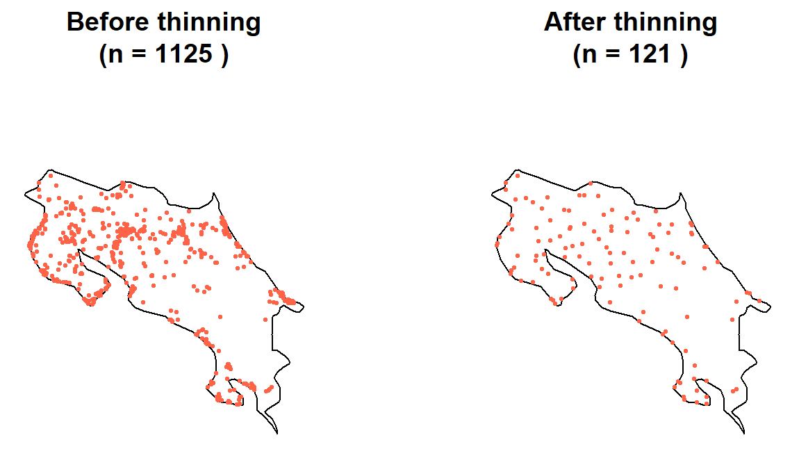
par(mfrow = c(1, 1))The thinned dataset should look less bunched. We’ve traded record volume for spatial representativeness, and because the raster resolution sets the limit on what environmental information is recoverable anyway, we haven’t actually lost anything the model could have used (Boria et al. 2014).
Step 4: Generate background points
Our model needs a reference: what does “not specifically selected by the species” look like environmentally? For this, we generate background points — random locations across the study region.
Background points are sometimes called pseudo-absences. They’re not true absences (we don’t know the species is absent there), but they represent the range of environmental conditions available across the landscape. Without them, a model has no baseline to compare presence conditions against.
We sample from within the region polygon — the same
approach we used in Module 5 to generate random points.
set.seed(42)
n_bg  <- nrow(howler_thinned) * 5   # 5x presences is a common rule of thumb
bg_sf <- st_sample(region, size = n_bg)
bg_sf <- st_sf(geometry = bg_sf)

plot(st_geometry(region), main = "Presence (red) and background (grey) points")
plot(st_geometry(bg_sf), add = TRUE, col = adjustcolor("grey50", 0.4), pch = 19, cex = 0.3)
plot(st_geometry(howler_thinned), add = TRUE, col = "tomato", pch = 19, cex = 0.5)
legend("bottomleft", legend = c("Presence", "Background"),
       col = c("tomato", "grey50"), pch = 19, bty = "n")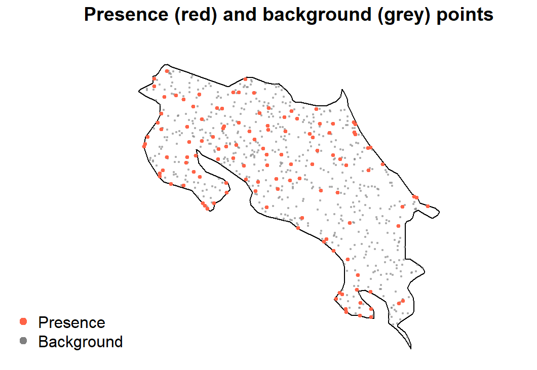
The 5× ratio is a reasonable starting point; some studies use 10× or more. The key is that background points sample broadly from available environmental space, not just areas near presences (Phillips et al. 2009).
Step 5: Extract environmental values
Now we extract environmental values at both presences and background points, creating the data frame that the model will actually learn from.
# Presence points
pres_vect   <- vect(howler_thinned)
pres_env    <- terra::extract(env_stack, pres_vect)
pres_coords <- as.data.frame(st_coordinates(howler_thinned))
names(pres_coords) <- c("x", "y")
pres_df <- data.frame(pres_coords, occ = 1, pres_env[, -1])

# Background points
bg_vect   <- vect(bg_sf)
bg_env    <- terra::extract(env_stack, bg_vect)
bg_coords <- as.data.frame(st_coordinates(bg_sf))
names(bg_coords) <- c("x", "y")
bg_df <- data.frame(bg_coords, occ = 0, bg_env[, -1])

# Combine and clean
howler_sdm <- rbind(pres_df, bg_df)
howler_sdm <- na.omit(howler_sdm)

nrow(howler_sdm)
## [1] 725table(howler_sdm$occ)##
## 0 1
## 605 120head(howler_sdm)## x y occ bio01 bio02 bio03 bio04 bio05 bio06
## 1 -85.73189 11.03608 1 26.31638 7.191382 71.24990 69.52401 31.83011 21.73693
## 2 -85.59351 11.12194 1 25.75554 7.619792 71.51208 72.19042 31.62700 20.97175
## 3 -84.72051 11.02987 1 26.20991 7.753187 73.59457 74.72079 31.76125 21.22625
## 4 -85.73476 10.95183 1 26.51744 8.294092 72.65295 73.01652 32.79776 21.38172
## 5 -85.61836 10.83835 1 25.83055 8.521063 72.60619 74.77908 32.34800 20.61200
## 6 -85.49022 10.85402 1 22.91079 8.188958 74.82088 69.78344 28.70600 17.76125
## bio07 bio08 bio09 bio10 bio11 bio12 bio13 bio14 bio15 bio16
## 1 10.09318 26.10009 26.91695 27.35275 25.56411 1739 345 5 87.74148 882
## 2 10.65525 25.55842 26.35017 26.80375 24.94571 1978 328 6 71.11481 873
## 3 10.53500 26.40621 26.67200 27.18171 25.27837 2607 361 43 53.89819 1030
## 4 11.41604 26.16182 26.59708 27.61306 25.78750 1658 340 1 94.26595 868
## 5 11.73600 25.49813 25.87858 26.93763 25.04779 1749 331 2 87.81650 865
## 6 10.94475 22.86354 23.31437 23.80442 22.05571 2694 366 39 50.67036 1013
## bio17 bio18 bio19 elev
## 1 33 210 193 116
## 2 55 224 338 221
## 3 163 282 629 38
## 4 9 223 129 144
## 5 17 240 165 259
## 6 180 296 675 683The occ column is what our model will predict: 1 =
presence, 0 = background. Every other column is an environmental
predictor.
Save your work
save(howler_thinned, bg_sf, howler_sdm, file = 'data/module7_occdata.RData')Exercise
- How many records were lost at each cleaning step — duplicates, imprecise coordinates, clipping to polygon, spatial thinning? Which step had the largest effect?
- Try running the clipping step (
st_within) before the duplicate removal step. Does the order matter? Why or why not? - Plot the thinned presence points on top of the
bio12(annual precipitation) raster. Do howler records appear to cluster in wetter areas, drier areas, or show no obvious pattern? - Change
n_bgto 10× the number of thinned presences. How doestable(howler_sdm$occ)change? Why might a very high ratio of background to presence points cause problems for a statistical model?
References
Boria, R.A., Olson, L.E., Goodman, S.M. & Anderson, R.P. (2014). Spatial filtering to reduce sampling bias can improve the performance of ecological niche models. Ecological Modelling, 275, 73–77.
Hijmans, R.J. & Elith, J. (2019). Species Distribution Modeling with R. CRAN vignette. Available at: https://rspatial.org/sdm/
Phillips, S.J., Dudík, M., Elith, J., Graham, C.H., Lehmann, A., Leathwick, J. & Ferrier, S. (2009). Sample selection bias and presence-only distribution models: implications for background and pseudo-absence data. Ecological Applications, 19, 181–197.