Building a species distribution model
For this module, you’ll need the following packages:
sfterracorrplot
In Module 8 we explored which environmental variables seem most associated with howler monkey occurrences. Now we formalise that into a species distribution model (SDM) that quantifies the relationship between environment and occurrence probability, and can be projected across the landscape to predict where the species is likely to be found.
SDMs have become one of the most widely used tools in ecology and conservation biology over the past two decades. They’ve been applied to assess climate change impacts on species ranges (Thomas et al. 2004), guide survey effort for undiscovered populations, identify priority areas for conservation, and predict invasive species spread. Getting to grips with even a simple SDM puts a powerful analytical framework in your hands.
Why a GLM?
Several algorithm families are used for SDMs, ranging from simple regression approaches to complex machine learning methods like MaxEnt, random forests, and boosted regression trees. We’ll use a Generalised Linear Model (GLM).
Why? GLMs are transparent, well-understood statistically, and produce interpretable coefficients. You can read the model and understand what it’s saying: “occurrence probability increases with temperature up to a point, then decreases.” More complex algorithms can produce better predictive performance but are harder to interpret and easier to overfit. Starting with a GLM gives a solid baseline and a clear understanding of the modelling process (Guisan et al. 2017).
The key distinction from ordinary linear regression is the link function. Our response variable is binary (0/1), so predicted values must stay between 0 and 1. The model estimates log-odds on an unbounded scale; we back-transform to get probabilities. This is also known as logistic regression.
Load your data
load('data/region.RData')
load('data/module7_occdata.RData')
env_stack <- terra::rast('data/env_stack.tif')

nrow(howler_sdm)
## [1] 725table(howler_sdm$occ)##
## 0 1
## 605 120Dealing with correlated variables
Before fitting, we need to address multicollinearity. Including two highly correlated predictors in a regression model is like asking someone to describe two things while wearing a blindfold on one eye; it’s technically possible but the result is unstable and hard to interpret. Coefficient estimates become unreliable, standard errors inflate, and the model can give very different answers with small changes in the data (Dormann et al. 2013).
library(corrplot)

# Spearman correlation matrix on all predictor variables
cor_mat <- cor(howler_sdm[, 4:ncol(howler_sdm)],
               method = 'spearman',
               use = 'complete.obs')

corrplot.mixed(cor_mat, tl.pos = 'lt',
               tl.cex = 0.6,
               number.cex = 0.5,
               addCoefasPercent = TRUE)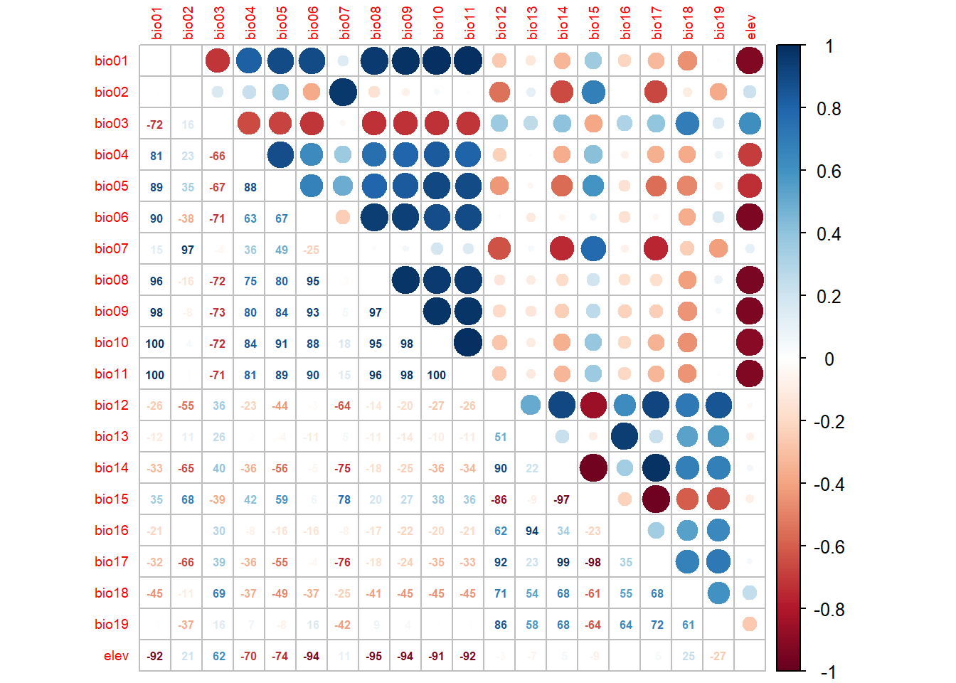
We’ll select variables by ranking them on individual predictive importance (AIC from a single-variable GLM), then working through the ranked list and dropping any variable that is too correlated (|r| > 0.7) with one already kept (Dormann et al. 2013).
# Step 1: rank all variables by univariate AIC (lower AIC = more important)
univar_aic <- sapply(names(howler_sdm)[4:ncol(howler_sdm)],
                     function(v) {
                       m <- glm(reformulate(v,
                                            response = 'occ'),
                                family = 'binomial',
                                data = howler_sdm)
  AIC(m)
})
univar_aic <- sort(univar_aic)

# Step 2: select weakly correlated subset
vars_ranked <- names(univar_aic)
pred_sel    <- c()

for (v in vars_ranked) {
  if (length(pred_sel) == 0) {
    pred_sel <- v
  } else {
    cors <- abs(cor_mat[v, pred_sel])
    if (all(cors < 0.7)) {
      pred_sel <- c(pred_sel, v)
    }
  }
}

pred_sel
## [1] "bio10" "bio18" "bio15" "bio02" "bio13" "bio19"p1 <- pred_sel[1]
p2 <- pred_sel[2]
cat("Top two predictors:", p1, "and", p2, "\n")## Top two predictors: bio10 and bio18Compare these top predictors to the ranking you calculated manually in Module 8. Do they agree?
Fitting your first SDM
The glm() function is built into R. We specify
family = "binomial" to indicate a binary response and the
logit link.
# Simple single-predictor model
m1 <- glm(reformulate(p1,
                      response = 'occ'),
          family = "binomial",
          data = howler_sdm)
summary(m1)
##
## Call:
## glm(formula = reformulate(p1, response = "occ"), family = "binomial",
## data = howler_sdm)
##
## Coefficients:
## Estimate Std. Error z value Pr(>|z|)
## (Intercept) -5.04046 1.01884 -4.947 7.53e-07 ***
## bio10 0.13433 0.03915 3.431 0.000601 ***
## ---
## Signif. codes: 0 '***' 0.001 '**' 0.01 '*' 0.05 '.' 0.1 ' ' 1
##
## (Dispersion parameter for binomial family taken to be 1)
##
## Null deviance: 650.62 on 724 degrees of freedom
## Residual deviance: 635.95 on 723 degrees of freedom
## AIC: 639.95
##
## Number of Fisher Scoring iterations: 5The summary gives us:
- Coefficients: the direction and magnitude of the relationship. A positive coefficient means occurrence probability increases with the variable; negative means it decreases.
- Null deviance: how poorly a model with no predictors fits the data.
- Residual deviance: how poorly our model fits — lower is better.
- AIC: model quality penalised for complexity. Lower AIC = better.
Explained deviance (D²) is the SDM analogue of R² in linear regression; the proportion of variation in the response accounted for by the model:
# Explained deviance: 1 - (residual deviance / null deviance)
1 - (deviance(m1) / m1$null.deviance)
## [1] 0.02256085Values above 0.1–0.15 are considered reasonable for SDMs; above 0.3 is quite good (Guisan & Zimmermann 2000).
More complex model structures
Species responses to environmental gradients are rarely linear. A species might prefer intermediate temperatures and decline at both extremes giving a hump-shaped (unimodal) response. We can capture this with a quadratic term.
# Quadratic model — allows a hump-shaped response
m1_q <- glm(
  as.formula(paste0("occ ~ ", p1, " + I(", p1, "^2)")),
  family = "binomial",
  data = howler_sdm
)
summary(m1_q)
##
## Call:
## glm(formula = as.formula(paste0("occ ~ ", p1, " + I(", p1, "^2)")),
## family = "binomial", data = howler_sdm)
##
## Coefficients:
## Estimate Std. Error z value Pr(>|z|)
## (Intercept) -5.726015 5.225758 -1.096 0.273
## bio10 0.194723 0.452128 0.431 0.667
## I(bio10^2) -0.001297 0.009659 -0.134 0.893
##
## (Dispersion parameter for binomial family taken to be 1)
##
## Null deviance: 650.62 on 724 degrees of freedom
## Residual deviance: 635.93 on 722 degrees of freedom
## AIC: 641.93
##
## Number of Fisher Scoring iterations: 51 - (deviance(m1_q) / m1_q$null.deviance)## [1] 0.02258906# Compare AIC: which fits better?
AIC(m1, m1_q)## df AIC
## m1 2 639.9458
## m1_q 3 641.9275A lower AIC for m1_q means the quadratic term is worth
including. Now let’s add a second predictor.
# Two predictors, both linear
m2 <- glm(
  as.formula(paste0("occ ~ ", p1, " + ", p2)),
  family = "binomial", data = howler_sdm
)
summary(m2)
##
## Call:
## glm(formula = as.formula(paste0("occ ~ ", p1, " + ", p2)), family = "binomial",
## data = howler_sdm)
##
## Coefficients:
## Estimate Std. Error z value Pr(>|z|)
## (Intercept) -4.7503090 1.2841354 -3.699 0.000216 ***
## bio10 0.1281961 0.0425033 3.016 0.002560 **
## bio18 -0.0002868 0.0007739 -0.371 0.710963
## ---
## Signif. codes: 0 '***' 0.001 '**' 0.01 '*' 0.05 '.' 0.1 ' ' 1
##
## (Dispersion parameter for binomial family taken to be 1)
##
## Null deviance: 650.62 on 724 degrees of freedom
## Residual deviance: 635.81 on 722 degrees of freedom
## AIC: 641.81
##
## Number of Fisher Scoring iterations: 51 - (deviance(m2) / m2$null.deviance)## [1] 0.02277233Stepwise model simplification
We’ll now fit a full model with linear and quadratic terms for both
top predictors, then use step() to simplify it. Stepwise
selection adds and drops terms based on AIC at each step, removing
parameters that don’t improve fit. This is a pragmatic approach to
variable selection and helps guard against a model that generalises
poorly (Burnham & Anderson 2002).
m_full <- glm(
  as.formula(paste0(
    "occ ~ ", p1, " + I(", p1, "^2) + ",
               p2, " + I(", p2, "^2)"
  )),
  family = 'binomial',
  data   = howler_sdm
)

summary(m_full)
##
## Call:
## glm(formula = as.formula(paste0("occ ~ ", p1, " + I(", p1, "^2) + ",
## p2, " + I(", p2, "^2)")), family = "binomial", data = howler_sdm)
##
## Coefficients:
## Estimate Std. Error z value Pr(>|z|)
## (Intercept) -4.565e+00 5.844e+00 -0.781 0.435
## bio10 6.835e-02 5.613e-01 0.122 0.903
## I(bio10^2) 1.254e-03 1.197e-02 0.105 0.917
## bio18 2.154e-03 6.316e-03 0.341 0.733
## I(bio18^2) -2.624e-06 6.725e-06 -0.390 0.696
##
## (Dispersion parameter for binomial family taken to be 1)
##
## Null deviance: 650.62 on 724 degrees of freedom
## Residual deviance: 635.63 on 720 degrees of freedom
## AIC: 645.63
##
## Number of Fisher Scoring iterations: 5AIC(m_full)## [1] 645.62931 - (deviance(m_full) / m_full$null.deviance)## [1] 0.02304733# Stepwise simplification
m_step <- step(m_full)## Start: AIC=645.63
## occ ~ bio10 + I(bio10^2) + bio18 + I(bio18^2)
##
## Df Deviance AIC
## - I(bio10^2) 1 635.64 643.64
## - bio10 1 635.64 643.64
## - bio18 1 635.75 643.75
## - I(bio18^2) 1 635.78 643.78
## <none> 635.63 645.63
##
## Step: AIC=643.64
## occ ~ bio10 + bio18 + I(bio18^2)
##
## Df Deviance AIC
## - bio18 1 635.76 641.76
## - I(bio18^2) 1 635.81 641.81
## <none> 635.64 643.64
## - bio10 1 645.55 651.55
##
## Step: AIC=641.76
## occ ~ bio10 + I(bio18^2)
##
## Df Deviance AIC
## - I(bio18^2) 1 635.95 639.95
## <none> 635.76 641.76
## - bio10 1 645.77 649.77
##
## Step: AIC=639.95
## occ ~ bio10
##
## Df Deviance AIC
## <none> 635.95 639.95
## - bio10 1 650.62 652.62summary(m_step)##
## Call:
## glm(formula = occ ~ bio10, family = "binomial", data = howler_sdm)
##
## Coefficients:
## Estimate Std. Error z value Pr(>|z|)
## (Intercept) -5.04046 1.01884 -4.947 7.53e-07 ***
## bio10 0.13433 0.03915 3.431 0.000601 ***
## ---
## Signif. codes: 0 '***' 0.001 '**' 0.01 '*' 0.05 '.' 0.1 ' ' 1
##
## (Dispersion parameter for binomial family taken to be 1)
##
## Null deviance: 650.62 on 724 degrees of freedom
## Residual deviance: 635.95 on 723 degrees of freedom
## AIC: 639.95
##
## Number of Fisher Scoring iterations: 5AIC(m_step)## [1] 639.94581 - (deviance(m_step) / m_step$null.deviance)## [1] 0.02256085Compare the full and simplified models. The simplified model should have lower or equal AIC — stepwise selection won’t simplify if doing so makes the model worse by this criterion. How much did the explained deviance change?
Save your work
my_preds <- c(p1, p2)
save(howler_sdm, pred_sel, p1, p2, my_preds, m_step, file = 'data/module9_sdm.RData')
Exercise
Using all variables in pred_sel (not just the top
two):
- Fit a full model with linear and quadratic terms for all selected
variables. You can build the formula string with
paste(paste0(pred_sel, " + I(", pred_sel, "^2)"), collapse = " + "). - Simplify it with
step(). - Compare the full and simplified models using
AIC()and explained deviance.
- Which model has lower AIC?
- Is the gain in explained deviance worth the additional complexity of the full model?
References
Burnham, K.P. & Anderson, D.R. (2002). Model Selection and Multimodel Inference: A Practical Information-Theoretic Approach. 2nd edition. Springer, New York.
Dormann, C.F., Elith, J., Bacher, S., Buchmann, C., Carl, G., Carré, G., Marquéz, J.R.G., Gruber, B., Lafourcade, B., Leitão, P.J., Münkemüller, T., McClean, C., Osborne, P.E., Reineking, B., Schröder, B., Skidmore, A.K., Zurell, D. & Lautenbach, S. (2013). Collinearity: a review of methods to deal with it and a simulation study evaluating their performance. Ecography, 36, 27–46.
Guisan, A. & Zimmermann, N.E. (2000). Predictive habitat distribution models in ecology. Ecological Modelling, 135, 147–186.
Guisan, A., Thuiller, W. & Zimmermann, N.E. (2017). Habitat Suitability and Distribution Models: With Applications in R. Cambridge University Press, Cambridge.
Thomas, C.D., Cameron, A., Green, R.E., Bakkenes, M., Beaumont, L.J., Collingham, Y.C., Erasmus, B.F.N., de Siqueira, M.F., Grainger, A., Hannah, L., Hughes, L., Huntley, B., van Jaarsveld, A.S., Midgley, G.F., Miles, L., Ortega-Huerta, M.A., Peterson, A.T., Phillips, O.L. & Williams, S.E. (2004). Extinction risk from climate change. Nature, 427, 145–148.